
Concentration of Measure: The Glorious Chernoff Bound
..and how to derive it


Suppose that we have n fair coins, and we decide to toss them, one by one, and count the number X of HEADS that we see. What can we say about this number X? This is the main question we will try to answer here.

To start, we index the coins from 1 to n and define the random variable Xᵢ to be equal to 1 if the i-th coin toss turns out to be HEADS, and 0 otherwise.
Clearly, for every i = 1, …, n, we have that Pr[Xᵢ = 1] = 1/2.
The above definition immediately gives
X = X₁ + X₂ + … + Xₙ.
The first step we can do is compute the expected value of X. We do this by exploiting the very useful property known as Linearity of Expectation, which states that the expected value of a sum of random variables (not necessarily independent) is equal to the sum of the corresponding expected values. Thus, we can write
E[X] = E[ X₁ + X₂ + … + Xₙ ] = E[X₁] + E[X₂] + … + E[Xₙ] = n/2,
where we used the fact that for every i, we have
E[Xᵢ] = 1 * Pr[Xᵢ = 1] + 0 * Pr[Xᵢ = 0] = 1/2.
We conclude that the expected number of HEADS we will see is n/2.
One could, potentially, be already happy with this result. But we are not! A natural question, in our opinion, now to ask is about the probability of seeing a number of HEADS that is “close enough” to this expected value. In other words:
What is the probability that the value of X is close to its expected value?
To answer this question, we will utilize the famous Chernoff bound, which, quoting Wikipedia:
…is named after Herman Chernoff but due to Herman Rubin, and gives exponentially decreasing bounds on tail distributions of sums of independent random variables. It is a sharper bound than the known first- or second-moment-based tail bounds such as Markov’s inequality or Chebyshev’s inequality, which only yield power-law bounds on tail decay.
Note: The interested reader can first read here about what Markov’s inequality gives when applied to the problem in question.
What is the Chernoff Bound?
Informally, the Chernoff bound gives strong concentration results for sums of independent random variables. We will only focus on the case of sums of 0/1random variables, like the ones in our motivating question. So, we consider exactly the setting that we described above.
We are interested in showing strong concentration around the expected value, and so we will focus on the probability of the following events:
- Pr[ X ≥ (1 + δ) μ ], and
- Pr[ X ≤ (1 - δ) μ ],
where δ > 0 is a small real number and μ = E[X] = n/2 is a short-hand notation for the expected value of X.
As a reminder, we first state Markov’s inequality.
Markov’s inequality: Let X be a non-negative random variable, and let A > 0 be a positive real number. Then, we have Pr[ X ≥ A] ≤ E[X] / A.
We are ready to start. We introduce a positive real parameter t > 0, which will be specified later on, and we write
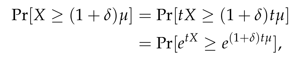
where we used the fact that t > 0, and that the exponential function is strictly increasing. We now apply Markov’s inequality and obtain
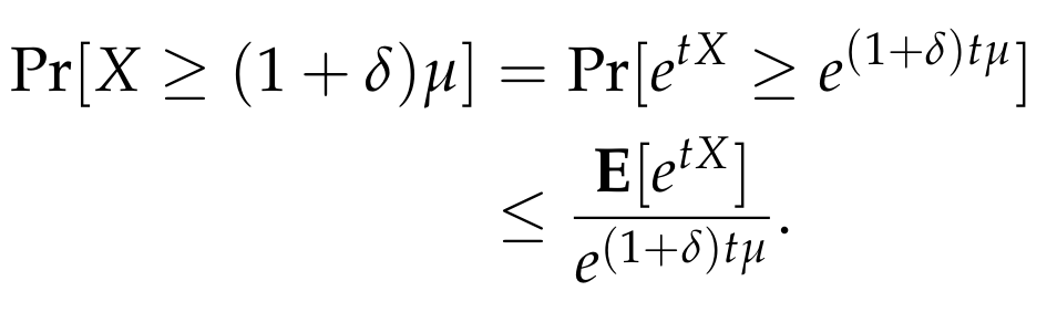
We now focus on the numerator of the right-hand side and get
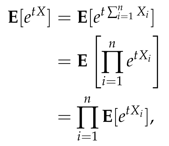
where in the last step we used the fact that the variables {Xᵢ} are independent. Each term in the product above can be easily computed as follows.
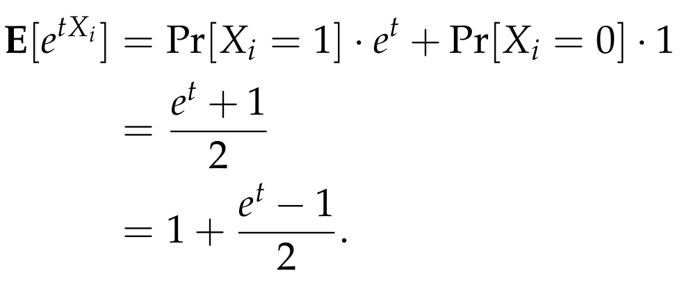
The reason that we wrote it in this form is that we would like now to apply the very useful inequality that states that for any real number x, we have
1 + x ≤ eˣ.
Applying this inequality, we get that
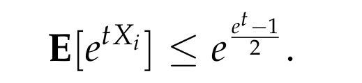
Thus, we get that
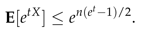
Putting everything together, we conclude that
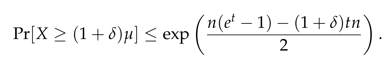
Since t > 0 is a free parameter, our goal is to pick its value in such a way so as to minimize the right-hand side. The exponential function is strictly increasing, so to minimize the right-hand size, we have to minimize the exponent
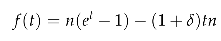
which is treated as a function f of t. The first derivative of f, with respect to t, is

which implies that the function is minimized for t = ln (1 + δ). Substituting this value of t in the above bound gives
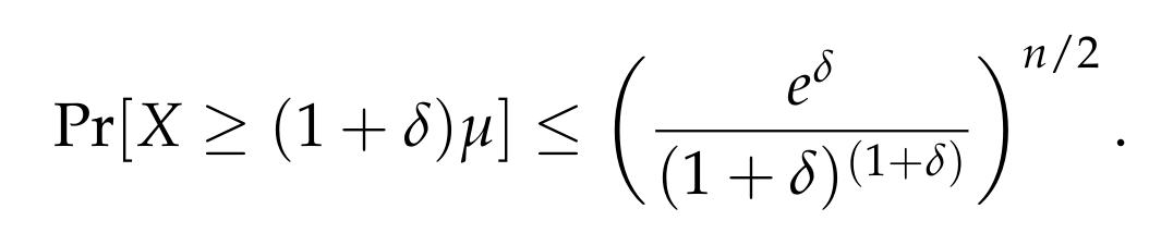
And here we have it, the Chernoff bound!
Of course, the above expression might be a bit complicated to parse, so we can get a slightly looser but simpler bound by using the following fact.
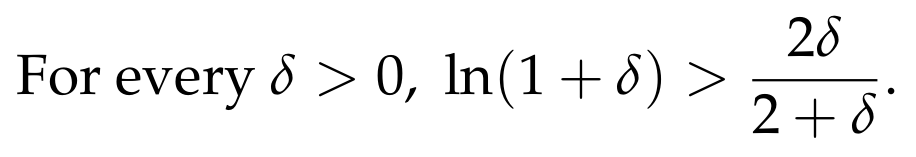
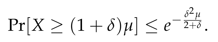
We will not prove the above fact, but the interested reader is suggested to do so. We now return to the right-hand side of the Chernoff bound and write

Thus, we conclude with the following form of the Chernoff bound, which holds for every δ > 0:
Finally, if we focus on small values of δ, and in particular, if 0 < δ < 1, then we can obtain the following form of the Chernoff bound.

The above theorem generalizes the discussion above in two ways:
- The coin flips are allowed to be biased, and the probability of each coin of getting a HEADS is some real number p that belongs in the [0,1] interval. The analysis above applies immediately to this more general case.
- Modifying the above analysis, we can also get a similar bound for the probability that X is smaller than (1 - δ)μ, as described in the theorem.
Back to coin flips
Going back to our original question, we can apply the above theorem and conclude that for any given 0 < δ < 1, we have
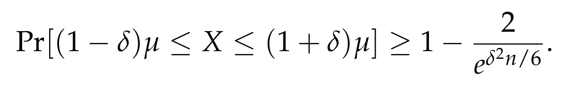
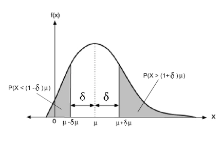
This shows that as the number n of coins increases, the probability that we are far from the expected value tends exponentially fast to 0. Thus, roughly speaking, the overwhelming mass of the random variable X is concentrated in a small interval [μ - δμ, μ + δμ] around the expected value μ! This is a very strong result, much more satisfying compared to the one we could have obtained by using Markov’s or Chebyshev’s inequality. Pictorially, it can be described as follows.
Conclusion
Concentration of measure is a very useful phenomenon that is exploited in many areas, such as statistics, randomized algorithms, machine learning, and more; one particularly beautiful application of concentration of measure that we discussed in the past is about dimensionality reduction in Euclidean spaces and can be found here. The Chernoff bound is one of the main ways of quantifying this concentration, and shows up in many different applications (see, e.g., the applications described here). Using Chernoff bounds, we can show that estimates we derive are very close to the actual values in question, that algorithms succeed with high probability, and many more.

Chernoff bounds can also be derived in cases where the given random variables are not independent, but are, for example, negatively correlated. In general, the theory of concentration of measure is very rich and the interested reader is encouraged to explore the many sources that are available online.
To sum up, Chernoff bounds are extremely useful, can be used in many different scenarios, and so it is always useful to keep them in mind!


