In probability theory and statistics, Markov’s inequality gives an upper bound for the probability that a non-negative function of a random variable is greater than or equal to some positive constant.

The inequality is named after Russian mathematician Andrey Markov (1856–1922) and is useful for relating probabilities to expectation by providing bounds for cumulative distribution of a stochastic variable.

Introduction

Suppose that you are tossing N coins, one after the other. A first natural question to ask is “what is roughly the number of HEADS you should expect to see?”. Well, if we assume that the coin flips are independent and unbiased, then on expectation you should see N/2 HEADS. OK, that seems reasonable so far.

So, let’s ask a second question: “how likely is it to see more than 2N/3 HEADS?” First, we note that it is definitely possible to observe at least 2N/3 HEADS, so the probability of such an event is positive. But, is there a way to bound such a probability? The answer is YES, and the simplest way to do so is by using the elegant Markov’s inequality.

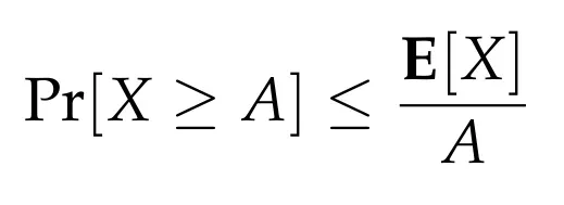
The starting point for Markov’s inequality to apply is a random variable X that is non-negative. In our case, X represents the number of HEADS we observe in Ncoin flips. Let E[X] denote the expected value of this random variable, and let A > 0 be some positive number. Then Markov’s inequality says that the probability of X taking value at least as large as A is at most E[X]/A. Formally,

That’s it!

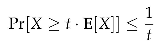
It is important to observe here that Markov’s inequality is interesting when one wants to compute how larger a random variable can get compared to its expected value. In particular, it directly gives the following bound, for any positive number t > 1:

An example

Before proving the inequality, let’s apply it to our example. We would like to get a bound on the probability that we observe at least 2N/3 HEADS in our N coin flips. As stated, it is easy to compute that E[X] = N/2. Thus, by applying Markov’s inequality, we get

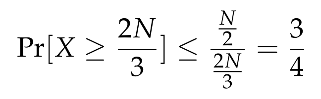
So, right away, this implies that with probability at least 1/4, we will observe fewer than 2N/3 HEADS, or equivalently, we will observe more than N/3 TAILS.

Let’s see now how one can prove Markov’s inequality.

The proof of Markov’s Inequality

The proof is surprisingly simple! We will use the definition of the expected value and the law of total probability, or more precisely, the law of total expectation. We have

Since X is always non-negative, we immediately have that E[X | X< A] ≥ 0. Thus, the first term on the right-hand side of the equality is always non-negative. Let’s ignore this term, and get that

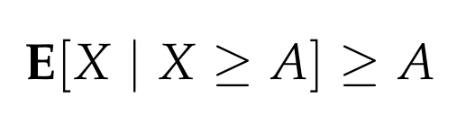
Almost there! The only observation we need to make is that when we condition the variable X to be at least A, then clearly, the expected value under this condition is always at least A. More formally,

Plugging this into the above inequality, we get that

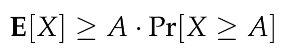
By rearranging the terms, we conclude that

Markov’s inequality is officially proved!

The great thing about Markov’s inequality is that, besides being so easy to prove, it is sometimes tight! And even if it is not, it still often gives very useful bounds.

Tightness of Markov’s inequality

A simple example that shows that the inequality is tight is the following. Let Z be random variable defined as follows.

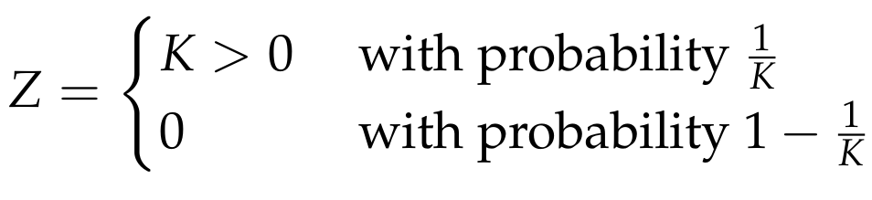
Note that its expected value is 1. Markov’s inequality now implies that

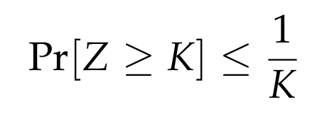
Indeed, the probability that Z is at least K is equal to the probability that Z is exactly K (as Z only takes values 0 and K), and this probability is equal to 1/K.

Conclusion

Markov’s inequality, although simple, is often very useful, and in many cases provides satisfactory bounds, especially when more sophisticated techniques cannot be applied (e.g., when we do not know much more for a random variable other than its expected value and the fact that it is always non-negative). Of course, there are cases where we can do a much better analysis (as in the example above with the independent coin flips, where one can apply more sophisticated techniques, as the Chernoff bound). Nevertheless, it is always good to keep it in mind, and, well, if you ever forget the statement, the proof is 2 minutes away!