Motion of a moving particle is considered to be one of the most instructive and useful physical systems one can study. In a real world case, such systems may exhibit immense complexity and intractability. But if we are lucky, we may be able to isolate the moving particle from unwanted effects coupled to the system, and may consider the system of a moving particle, a simple problem in physics.

The standard approach to completely solve the problem of a moving particle has been known for a very long time — the methods given to us by Isaac Newton. In modern literature, these methods employ simple but heavy use of calculus which are very efficient and effective, but using calculus sometimes might not the most physically intuitive approach.

In this article we are going to explore a non-calculus and (arguably) simpler approach to solve the problem of a moving particle.

The Moving Particle

Let us start with the simplest case — the particle moving with a speed that does not change with time, i.e. constant speed. In mathematical terms, it can be written as -

where s(t) is the speed of the particle at time t, whose value is s₀ which is set at the initial time t=0 and remains fixed for as long the system is under observation.

Here, we do not require any sophisticated mathematical skills to obtain the distance covered by such a particle in time t. We use the widely known fact-

Distance covered is equal to the speed multiplied by the time taken

In mathematical terms -

where d(t) is the distance covered by the particle moving with constant speed s₀in time t.

Things can quickly become significantly more difficult if we now allow the particle to move with a speed that changes with time. Such a motion is called an accelerated motion and the formula mentioned above does not work anymore! It is at this point, most standard textbooks begin to discuss and define acceleration via calculus.

Accelerated Motion

We are going to try and understand the idea of acceleration, without actually defining it with mathematical precision, but we will properly include the effects of the change in speeds, without loosing mathematical rigor.

Previously, we had obtained the expression of speed as -

If the speed of the particle changes with time, we must have a quantity on the right-hand-side, which captures this effect. The simplest way to include time-dependence is as follows -

Here, we have constructed an expression in which the dependence of time is linear, and a is just a parameter that quantifies the ‘strength’ of this dependence. We could find a better (and mathematically more accurate) name for this parameter — an acceleration factor.

It turns out that this construction is more than capable in solving a huge variety of simple practical problems, and we will return to this point later. But, if we decide to go further, we can include slightly more complicated time-dependence as follows -

This expression captures the linear effects of change in speed with time and a bit more. The strength of this extra dependence is quantified by another acceleration factor, a₂. We can keep adding such additional factors and the expression for speed will become more and more generalized. Let us take all such factors at once and see what we get -

This expression can be compactly written as -

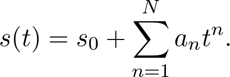
This particular form of the expression of speed is useful because we can recover the original constant-speed case by putting aₙ = 0 for all values of n.

We now have a very general expression of time-dependent speed of a moving particle. But, we still need to find a corresponding expression for distance covered, and that is what we are going to do next.

By following a similar line of reasoning, we could try to write an expression and see if it works -

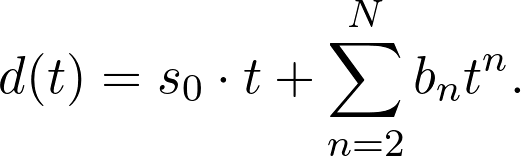
In this expression, we have chosen a different set of acceleration factors, namely bₙ. This is required because we do not yet know that we can use the same acceleration factors for obtaining the distance covered. If we are lucky, they might turn out to be equal. Another important point is that the starting value of n is equal to 2, and not 1 as before. This is because n=1 would correspond to a factor linear in time like b₁⋅ t, and we already have such a term in s₀ ⋅ t.

To make the expression look slightly more consistent, we may rewrite it as -

This is still the same expression, except that it will offer some mathematical simplifications later on.

Finding The Distance Covered

Our goal now is to establish a relationship between acceleration factors aₙ and bₙ. In order to do that, we use a very simple physical observation.

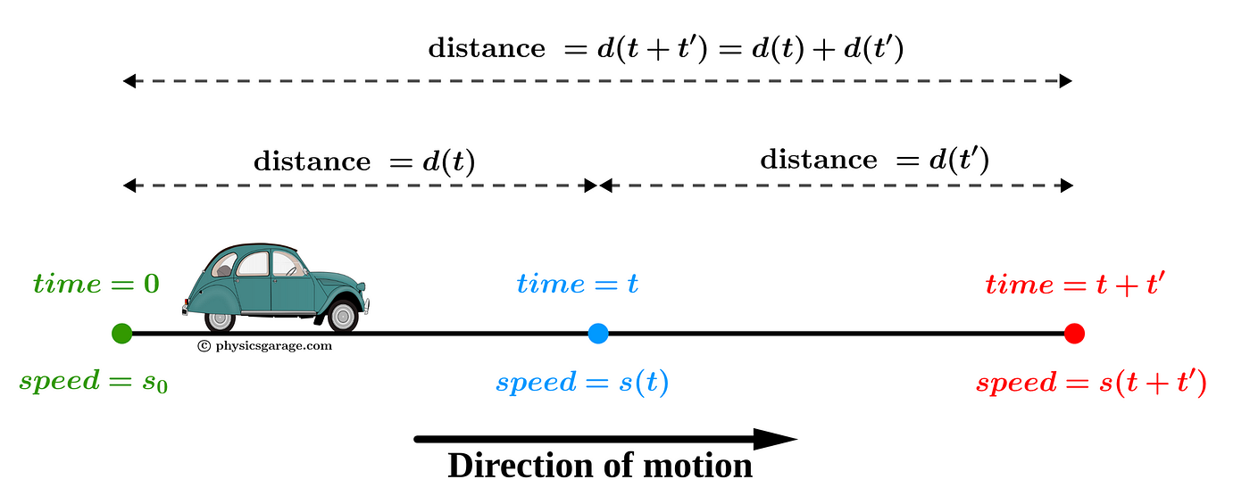
Let us imagine a moving particle covers a distance of 100 meters in 10 seconds in one go and ends its journey. The important point is that, we are not specifying anything about it’s speed; it could be moving with a fixed speed throughout, or with a speed that changes with time in an arbitrary manner. Now, let us say imagine a different way to cover the same distance. Imagine that the particle starts with a speed of 2 meters-per-second and covers the first 80 meters in 6seconds, while changing its speed along the way. It is obvious that the remaining 20 meters of the journey must be covered in 4 seconds, now starting with the speed that the particle had acquired at the end of 6 seconds. There are three important observations that we are trying to understand:

1. We can split the entire journey in two parts (or more), and still have the same end result.
2. It does not matter how we split the time interval, the distance covered should still be the same.
3. An exact description of the time-dependence of speed doesn’t seem to play a role, as long as we can obtain the values of speeds at the beginning and at the interval split. The intermediate values are not explicitly needed!

To write this in mathematical form, let us imagine that the total time taken by the particle starting with a speed of s₀ to cover a certain distance is (t+t′), and we split the journey at time t.

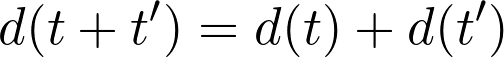
So, we have -

We already know the expression for d(t) on the right-hand-side as -

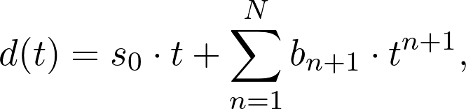
which can be used to obtain the expression of d(t+t′) as -

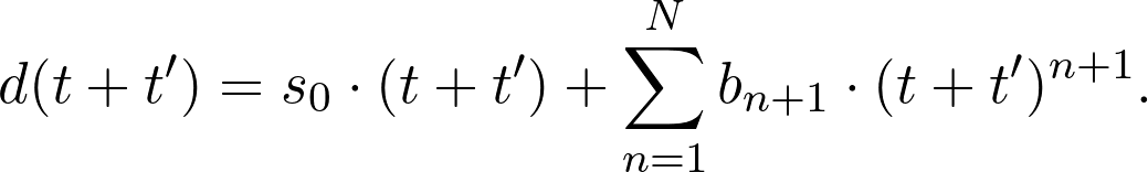
We can again use this to obtain the expression of d(t′), except that now we have to use the value of speed at the end of time t. To obtain this value, we recall the expression of the time-dependent speed -

This is the value of ‘initial speed’ that we should be using for the journey that starts at the end of time t, instead of s₀. So, we get -

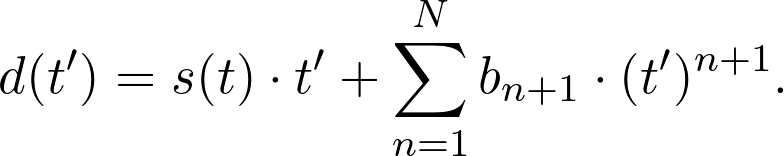
And, if we substitute the expression for s(t), we get -

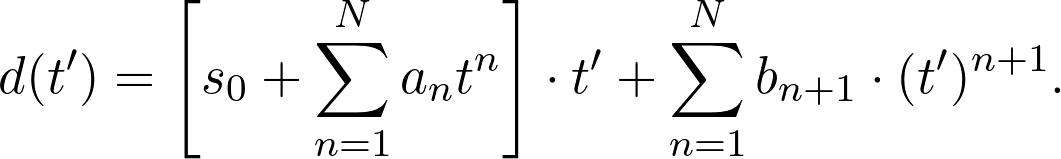
Putting it all together, we obtain one scary looking expression -

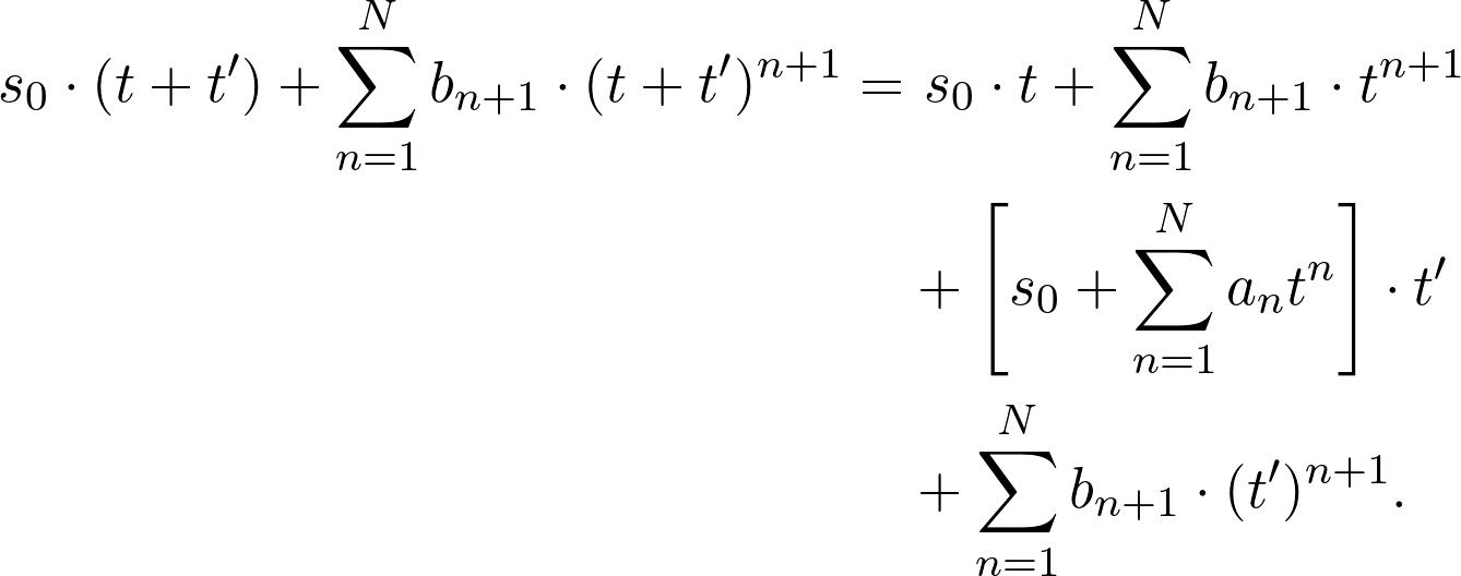
Fortunately, we can reduce this equation significantly. After cancelling out common factors involving s₀ on both sides, we get -

To further simplify this expression, we use the binomial theorem -

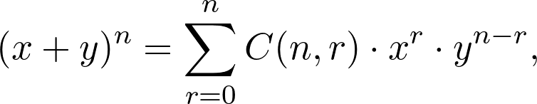
with

We use this on the factor (t+t′)ⁿ⁺ ¹ to get -

Again, this scary looking expression can be much simplified. If we want to compare the coefficients of tⁿ⁺ ¹ on both side, we must choose r=n+1 on the left-hand-side to get -

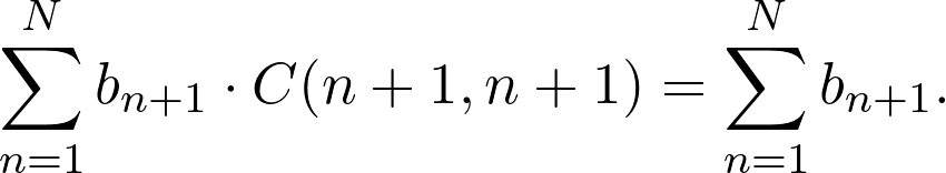
It can easily be evaluated to see that C(n+1, n+1) = 1, so that the terms on both sides are equal and hence can be cancelled with each other. A similar cancellation occurs if we compare the coefficients of (t′)ⁿ⁺ ¹ by choosing r=0. After all the cancellations we are left with a simpler looking expression -

One last simplification can also be done by comparing the coefficients of t′ by choosing r=n to get -

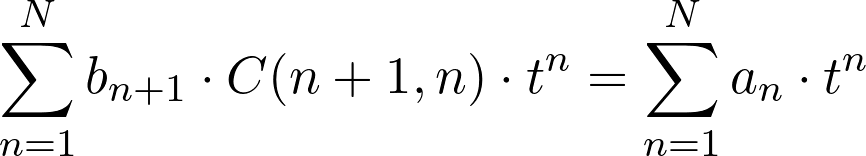
Since the point of splitting the journey is arbitrary, t can take any value, and this equality is valid only if we have -

By a simple rearrangement we can write this as -

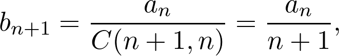
where the second equality comes from the definition of C(n, r) as given before.

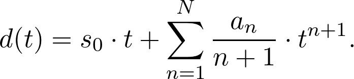
This is the relationship between the acceleration factors used in speed of the particle and the distance covered by it. By substituting the expression of bₙ₊₁, we can finally write the expression of speed and distance as -

Special Case

As promised earlier, we can now obtain these expressions for the case when aₙ = 0for n>1. By choosing n= 1 and a₁ = a, we get -

These are exactly the same expressions that one would obtain by using the standard calculus based methods.

Want to read more stories like this?

• Originally published at https://physicsgarage.com on March 10, 2021.