Introduction to Group Theory

Imagine a square of paper lying flat on your desk. I ask you to close your eyes. You hear the paper shift. When you open your eyes the paper doesn’t appear to have changed. What could I have done to it while you weren’t looking?

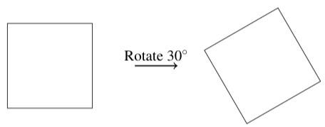
It’s obvious that I haven’t rotated the paper by 30 degrees, because then the paper would look different.

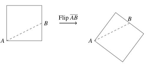
I also did not flip it over across a line connecting, say, one of the corners to the midpoint of another edge. The paper would look different if I had.

What I could have done, however, was rotate the paper clockwise or counterclockwise by any multiple of 90 degrees, or flipped it across either of the diagonal lines or the horizontal and vertical lines.

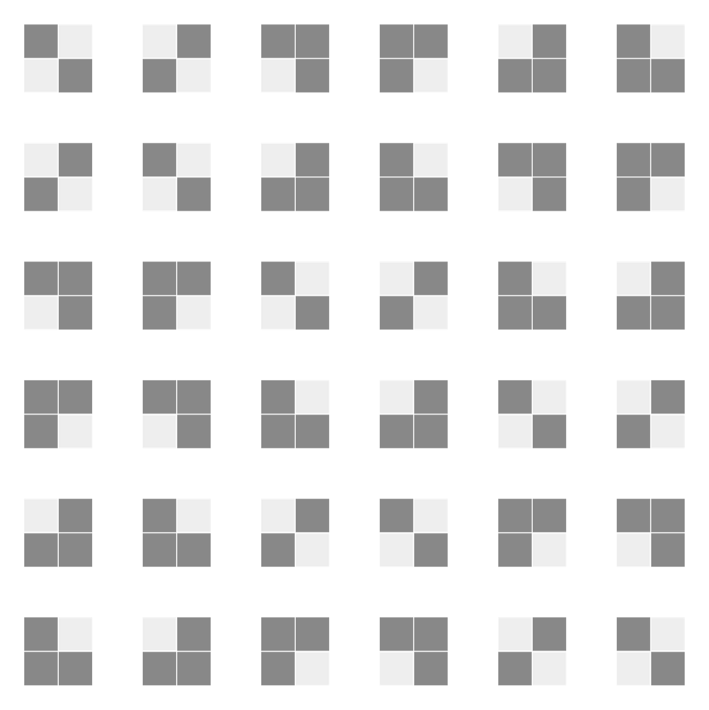
A helpful way to visualize the transformations is to mark the corners of the square.

The last option is that to do nothing. This is called the identity transformation. Together, these are all called the symmetry transformations of the square.

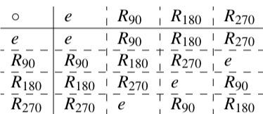
I can combine symmetry transformations to make other symmetry transformations. For example, two flips across the line segment BD produces the identity, as do four successive 90 degree counterclockwise rotations. A flip about the vertical line followed by a flip about the horizontal line has the safe effect as a 180 degree rotation. In general, any combination of symmetry transformations will produce a symmetry transformation. The following table gives the rules for composing symmetry transformations:

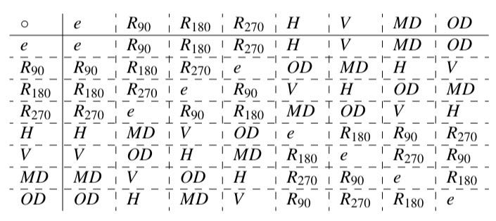
In this table, R with subscripts 90, 180, and 270 denote counterclockwise rotations by 90, 180, and 270 degrees, H means a flip about the horizontal line, V is a flip about the vertical line, MD is a flip about the diagonal from the top left to the bottom right, and OD means a flip over the other diagonal. To find the product of A and B, go to the row of A and then over to the column of B. For example, H∘MD=R₉₀.

There are a few things you may notice by looking at the table:

• The operation ∘ is associative, meaning that A∘(B∘C) = (A∘B)∘C for any transformations A, B, and C.
• For any pair of symmetry transformations A and B, the composition A∘B is also a symmetry transformation
• There is one element e such that A∘e=e∘A for every A
• For every symmetry transformation A, there is a unique symmetry transformation A⁻¹ such that A∘A⁻¹=A⁻¹∘A=e

We therefore say that the collection of symmetry transformations of a square, combined with composition, forms a mathematical structure called a group. This group is called D₄, the dihedral group for the square. These structures are the subject of this article.

Definition of a group

A group ⟨G,*⟩ is a set G with a rule * for combining any two elements in G that satisfies the group axioms:

• Associativity: (a*b)*c = a*(b*c) for all a,b,c∈G
• Closure: a*b∈G all a,b∈G
• Unique identity: There is exactly one element e∈G such that a*e=e*a=a for all a∈G
• Unique inverses: For each a∈G there is exactly one a⁻¹∈G for which a*a⁻¹=a⁻¹*a=e.

In the abstract we often suppress * and write a*b as ab and refer to * as multiplication.

It is not necessary for * to be commutative, meaning that a*b=b*a. You can see this by looking at the table of D₄, where H∘MD=R₉₀ but MD∘H=R₂₇₀. Groups where * is commutative are called abelian groups after Neils Abel.

Abelian groups are the exception rather than the rule. Another example of a non-abelian group is the symmetry transformations of a cube. Consider just rotations about the axes:

If I first rotate 90 degrees counterclockwise about the y-axis and then 90 degrees counterclockwise about the z-axis then his will have a different result than if I were to rotate 90 degrees about the z-axis and then 90 degrees about the y-axis.

It is possible for an element to be its own inverse. Consider the group which consists of 0 and 1 with the operation of binary addition. Its table is:

Clearly 1 is its own inverse. This is also an abelian group. Don’t worry, most groups aren’t this boring.

Some more examples of groups include:

• The set of integers with addition.
• The set of rational numbers not including 0 with multiplication.
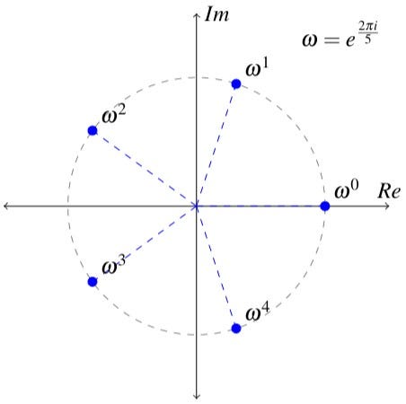
• The set of solutions to the polynomial equation xⁿ-1=0, called the nth roots of unity, with multiplication.

Here are some examples that are not groups:

• The set of natural numbers under addition is not a group because there are no inverses, which would be the negative numbers.
• The set of all rational numbers including 0 with multiplication is not a group because there is no rational number q for which 0/q=1, so not every element has an inverse.

Group structure

A group is a lot more than just a blob that satisfies the four axioms. A group can have internal structure, and this structure can be very intricate. One of the basic problems in abstract algebra is to determine what the internal structure of a group looks like, since in the real world the groups that are actually studied are much larger and more complicated than the simple examples we’ve given here.

One of the basic types of internal structure is a subgroup. A group G has a subgroup H when H is a subset of G and:

• For a,b∈H, a*b∈H and b*a∈H
• For a∈H, a⁻¹∈H
• The identity is an element of H

If H≠G then H is said to be a proper subgroup. The subgroup of G consisting only of the identity is called the trivial subgroup.

A group of n elements where every element is obtained by raising one element to an integer power, {e, a, a², …, aⁿ⁻¹}, where e=a⁰=aⁿ, is called a cyclic group of order n generated by a. Consider the cyclic subgroup of order 6, {e,a,a²,a³,a⁴,a⁵}. Its proper subgroups are {e,a³} and {e,a²,a⁴}.

A non-abelian group may have commutative subgroups. Consider the square dihedral group that we discussed in the introduction. This group is not abelian but the subgroup of rotations is abelian and cyclic:

We now give two examples of group structure.

Even if a group G is not abelian, it may still be the case that there is a collection of elements of G that commute with everything in G. This collection is called the center of G. The center C is a subgroup of G. Proof:

• Identity: eg=ge for all g∈G so e∈G.
• Closure: Let a,b∈C. By definition, ag=ga and bg=gb for all g∈G. So (ab)g=agb=g(ab), therefore ab commutes with all g∈G so ab∈C.
• Inverses: If a∈C then ga=ag for all g∈G, so a⁻¹(ga)a⁻¹=a⁻¹(ag)a⁻¹. By associativity, this means that a⁻¹g(aa⁻¹)=(a⁻¹a)ga⁻¹. Since aa⁻¹=a⁻¹a=e it follows that a⁻¹g=ga⁻¹ so a⁻¹∈C. QED.

Now suppose that f is a function whose domain and range are both G. A period of fis an element a∈G such that f(x)=f(ax) for all x∈G. The set P of periods of f is a subgroup of G. Proof:

• Identity: x=ex so f(x)=f(ex) for all x∈G therefore e∈P
• Closure: Let a,b∈P. Since bx∈G and f(x)=f(ax) for all elements of G, it follows that f(bx)=f(abx). But f(bx)=f(x) so f(x)=f(abx) therefore ab∈P.
• Inverses: Let a∈P. Then f(x)=f(ex)=f(a(a⁻¹x))=f(a⁻¹x) so a⁻¹∈P for. QED.

Finite groups are finitely generated

We saw that cyclic groups are generated by a single element. When it’s possible to write every element of a group G as products of a (not necessarily proper) subset A of G then we say that A generates G and write this as G=⟨A⟩. The most “well, duh” proof you’ll ever see is the proof that all finite groups are generated by a finite generating set:

• Let G be finite. Every element of G is a product of two other elements of G so G=⟨G⟩. QED.

Every finite group is trivially generated by itself but it may also be generated by a proper subset. For example, the group G={e, a, b, b², ab, ab²} with the constraints a²=e, b³=e, ba=ab² is is generated by a and b so G=⟨{a,b}⟩.

We will finish off this article with an application.

Error-resistant communication

The simplest way to transmit digital information is to encode it into binary strings of fixed length. No communication scheme is completely free from interference so there is always a possibility that the wrong data will be received. The method of maximum-likelihood decoding is a simple and effective approach to detecting and correcting transmission errors.

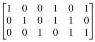
Let 𝔹ⁿ be the set of binary strings, or words, of length n. It is straightforward to show that 𝔹ⁿ is an abelian group under binary addition without carrying (so that for example 010+011=001). Note that every element is its own inverse. A code C is a subset of 𝔹ⁿ. The following is an example of a code in 𝔹⁶:

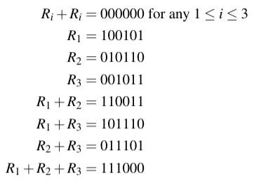
C = {000000, 001011, 010110, 011101, 100101, 101110, 110011, 111000}

The elements of a code are called codewords. Only codewords will be transmitted. An error is said to occur when interference changes a bit in a transmitted word. The distance d(a,b) between two codewords a and b is the number of digits in which two codewords differ. The minimum distance of a code is the smallest distance between any two of its codewords. For the example code just above, the minimum distance is three.

In the method of maximum-likelihood decoding, if we receive a word x, which may contain errors, the receiver should interpret x as the codeword a such that d(a,x) is a minimum. I will show that for a code of minimum distance m this can always (1) detect errors that change fewer than m bits and (2) correct errors that change ½(m-1) or fewer bits.

• 1: Suppose that the transmitter sends codeword p and that the codeword experiences an error that flips fewer than m bits, producing codeword q. Since d(p,q)<m, q cannot be a codeword so the receiver detects an error.
• 2: Define the sphere of radius k about a codeword a, written Sₖ(a), to mean all x∈𝔹ⁿ with d(a,x)≤k. Let a and b be codewords and suppose that k=½(m-1) and x∈Sₖ(a). The distance between the “centers” of Sₖ(a) and Sₖ(b) is at least m. If x∈Sₖ(a) then d(a,x)≤½(m-1) so d(b,x)≥m-½(m-1) therefore d(b,x)≥½(m+1) so x∉Sₖ(b). So if d(a,x)≤½(m-1) then a is the codeword of minimum distance from x so the receiver interprets x as a.

In our example code, m=3 and the sphere of radius ½(m-1)=1 about the codeword 011101 is {011101, 111101, 001101, 011001, 010101, 011111, 011100}. So if the receiver receives any of these words, it knows that it was supposed to receive 011101.

So that’s all well and good, but what does any of this have to do with group theory? The answer is in how we actually produce the codes that this method works with.

It is possible for a code in 𝔹ⁿ to form a subgroup. In this case we say that the code is a group code. Group codes are finite groups so they are finitely generated. We will see how to produce a code by finding a generating set.

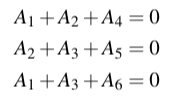
A code can be specified so that the first few bits of each codeword are called the information bits and the bits at the end are called the parity bits. In our example code C, the first three bits are information bits and the last three are parity bits. The parity bits satisfy parity-check equations. For a codeword A₁A₂A₃A₄A₅A₆ the parity equations are A₄=A₁+A₂, A₅=A₂+A₃, and A₆=A₁+A₃. Parity equations provide another layer of protection against errors: if any of the parity equations aren’t satisfied then an error has occurred.

Here is what we do. Suppose that we want codewords with m information bits and n parity bits. To generate a group code, write a matrix with m rows and m+n columns. In the block formed by the first m columns, write the m×m identity matrix. In column j for m+1≤j≤m_n, write a 1 in the kth row if Aₖ appears in the parity equation for parity bit Aⱼ and 0 otherwise. In our example code, the matrix is:

Such a matrix is called a generating matrix for the group code. You can verify directly that the rows generate C:

The rows of any generating matrix form a generating set for a group code C. Proof:

• Identity and inverses: Any row added to itself gives the identity, a string consisting of all zeros.
• Closure: If A,B∈C then A and B are sums of rows of the generating matrix so A+B is also a sum of rows of the generating matrix. Therefore A+B∈C.

This lets us generate a code, now I will show how to generate a useful code.

Define the weight w(x) to mean the number of ones in x. For example, w(100101)=3. It is obvious that w(x)=d(x,0) where 0 is a word whose digits are all zeroes. The minimum weight W of a code is the weight of the nonzero codeword with the fewest ones in the code. For a code of minimum distance m, d(x,0)≥m so w(x)≥m and therefore W=m.

Recall that for a word to be considered a codeword, it must satisfy a set of parity check equations. For our example code, these are A₄=A₁+A₂, A₅=A₂+A₃, and A₆=A₁+A₃. We can also write these as a linear system:

Which itself can be written in terms of dot products:

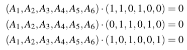
Or in more compact form as Ha=0 where a=(A₁,A₂,A₃,A₄,A₅,A₆) and H is the parity-check matrix for the code:

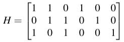
One can verify by direct computation that if w(a)≤2 then we cannot have Ha=0. In general, the minimum weight is t+1 where t is the smallest number such any collection of t columns of H do not sum to zero (i.e. they are linearly independent). Proving this would take us just a little bit too far into linear algebra.

If that frightens you, don’t worry. We can produce some very good codes without it by taking advantage of the fact that the result I just mentioned implies that if every column of H is nonzero and no two columns are equal then the minimum weight, and thus the minimum distance of the code, is at least three. This is very good: If our communication system is expected to have one bit error for every hundred words transmitted, then only one in ten thousand transmitted words will have an uncorrected error and one in one million transmitted words will have an undetected error.

So now we have a recipe for producing a useful code for the maximum-likelihood detection scheme for codewords containing m information bits and n parity bits:

• Create a matrix with m+n columns and n rows. Fill in the matrix with ones and zeros so that no two columns are the same and no column is just zeros.
• Each row of the resulting parity-check matrix corresponds to one of the parity bit equations. Write them as a system of equations and solve so that each parity bit is written in terms of the information bits.
• Create a matrix with m+n columns and m rows. In the block formed by the first m columns, write the m×m identity matrix. In column j for m+1≤j≤m_n, write a 1 in the kth row if Aₖ appears in the parity equation for parity bit Aⱼ and 0 otherwise.
• The rows of this matrix are the generators of a code group with minimum distance at least three. This is the code we will use.

As an example, suppose that I need a simple, eight-word code and I only need some basic error detection and not correction, so I can get away with a minimum distance of two. I want three information bits and two parity bits. I write down the following parity-check matrix:

There are two pairs of columns that are equal, so the smallest t for which any collection of t columns is linearly independent is one, so the minimum weight, and therefore the minimum distance I will have, is two. The rows represent the parity-check equations A₄=A₁+A₃ and A₅=A₁+A₂+A₃. My generating matrix is therefore:

And the rows of this matrix generate the code group:

• {00000, 00111, 01001, 01110, 10011, 10100, 111010, 11101}

Closing remarks

Abstract algebra is a deep subject with far-reaching implications, but it is also a very easy one to learn. Aside from a few passing mentions of linear algebra, nearly everything that I’ve discussed here is accessible to someone who’s only had high school algebra.

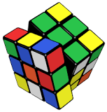
When I first had the idea to write this article I really wanted to talk about the Rubik’s cube, but in the end I wanted to pick an example that could be covered only with the most basic ideas in group theory. Plus, there is so much to say about the Rubik’s cube group that it deserves a standalone piece, so that will be coming soon.

My college courses in abstract algebra were based on the book A Book of Abstract Algebra by Charles Pinter, which is and accessible treatment. The examples in this article were all borrowed with some modification from Pinter.

As a final note, any images that are not cited are my own original work and may be used with attribution. As always, I appreciate any corrections or requests for clarification.