
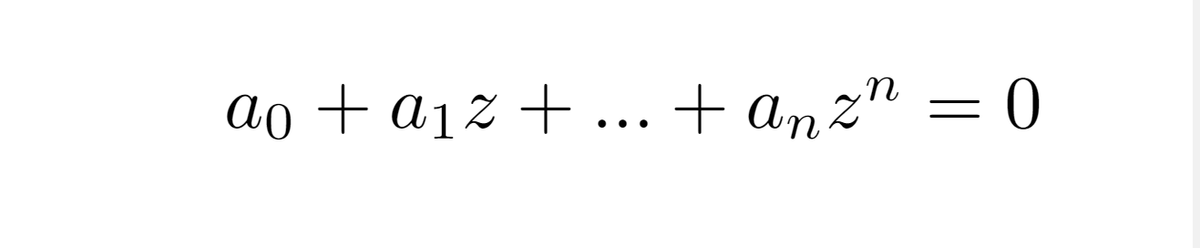
An Elementary Proof of the Fundamental Theorem of Algebra
Using only elementary methods we will prove the Fundamental Theorem of Algebra. Along the way, we’ll befriend some key ideas from…

Using only elementary methods we will prove the Fundamental Theorem of Algebra. Along the way, we’ll befriend some key ideas from elementary analysis and catch a glimpse into the beautiful world of complex numbers.

Motivation
Regardless of anything else, it’s been a great quarantine project for me:)
The aim of theory really is, to a great extent, that of systematically organizing past experience in such a way that the next generation, our students and their students and so on, will be able to absorb the essential aspects in as painless a way as possible, and this is the only way in which you can go on cumulatively building up any kind of scientific activity without eventually coming to a dead end.
Michael Atiyah, Fields Medalist, in ‘How research is carried out’
The language of elementary analysis is that of continuity, limits, open and closed sets, and of calculus in one variable. It is with hindsight we can see that these concepts and definitions reduce impossible problems into very doable. (Or, as I found, *doable* with intermittent attempts over several months and making many mistakes mistakes.)
In trying to prove this theorem, I used this language of elementary analysis. To begin with, you’ll get acquainted with what some of these (initially daunting) concepts mean. Then, we’ll use them to prove something which would otherwise seem impossible.
I’ve tried to include the bare minimum apparatus of what is needed. If you’re familiar with some of it, feel free to skip sections you’re familiar with. You can also get a feel for the proof and return to the pre-requisites as needed. Inevitably, if this is your first time meeting a lot of this material, don’t expect it all to make perfect sense; aim for understanding the gist of the argument, not every detail.
Statement of the Problem
Suppose we have a polynomial over the complex numbers, and we want to know if there is a complex number where the polynomial evaluates to 0. (An introduction to complex numbers can be found next, if needed)
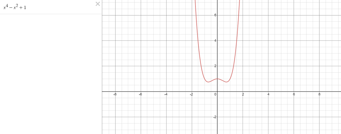
The Fundamental Theorem of Algebra states that every such polynomial over the complex numbers has at least one root. This is in stark contrast to the real numbers, where many polynomials have no roots, such as x² + 1. Over the complex numbers, z² + 1 has two roots: +i and -i. i²=-1 so both evaluate to -1+1 = 0.
In contrast, polynomials over the real numbers are not guaranteed to have at least one root. For example, the polynomial below doesn’t have any roots, as can be seen from its graph.
0. Gameplan
It is quite tricky to give the broad brushstrokes of what will be a somewhat technical proof. Please do not skip this section, as it is important to have an overarching view of what we are going to do!
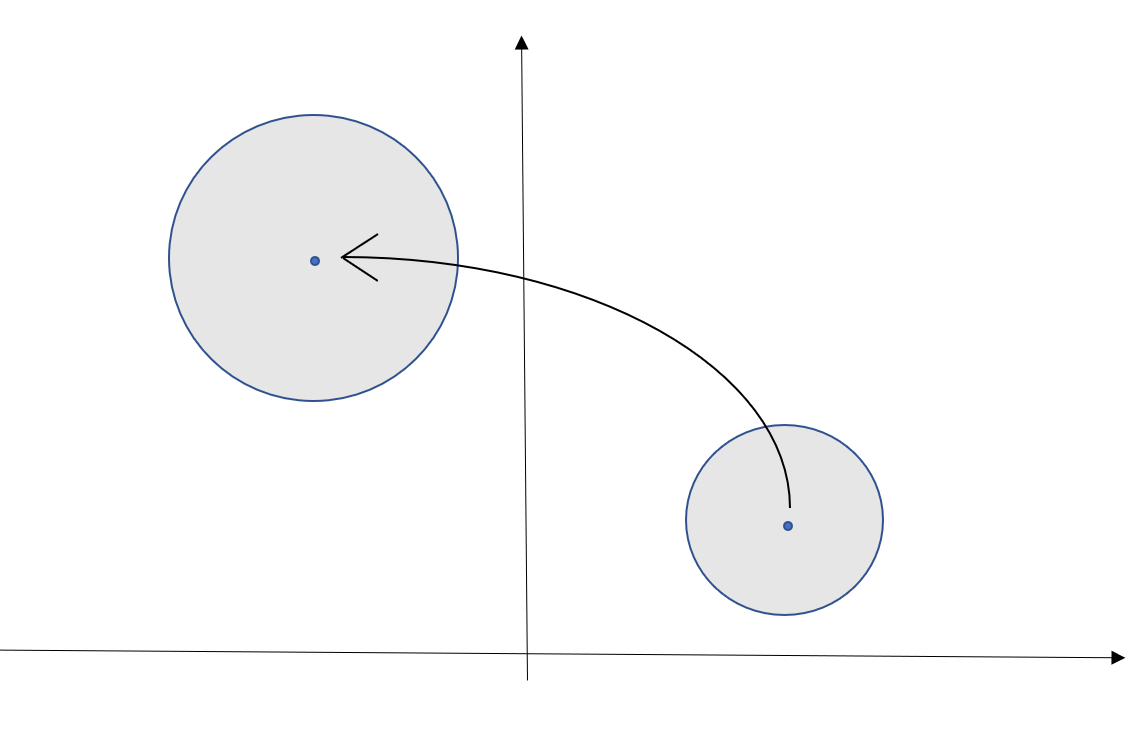
So, what I do here, is prove it for a very simple function. I prove it for P(z) = 2z, and I prove that P(z) = 2z has a root. Well, obviously it does, you say, just plug in P(0+0i) = 2(0+0i) = 0. Done.
But I’m going to pretend that I haven’t spotted this, and use a method which will generalise very nicely to more polynomials.
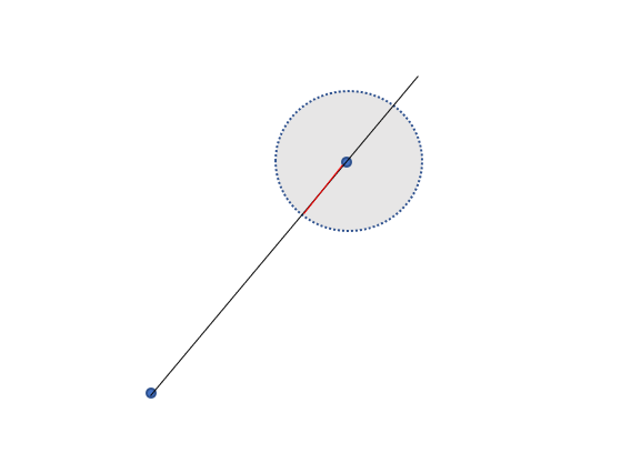
First, we take a point w. We can see where P sends w: P(w) = 2w. But what about in a small region around w? Draw a small circle around w in the complex plane, and see where all the points in it land. It turns out if we shaded in all the points where they landed it would form another circle.[Spoiler: when representing complex numbers, we do so in a 2D plane. That’s because z = x+iy can be represented as the coordinates (x,y) on a diagram]
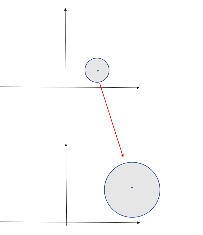
Now, suppose that for every complex number w except a finite number, say, 4 points, we could draw a shaded circle around w, then see where that lands, and finally we could inscribe a circle inside the ‘image’ of where that circle lands. A diagram shows the process of inscribing a circle inside the ‘image’ of where our old circle landed.
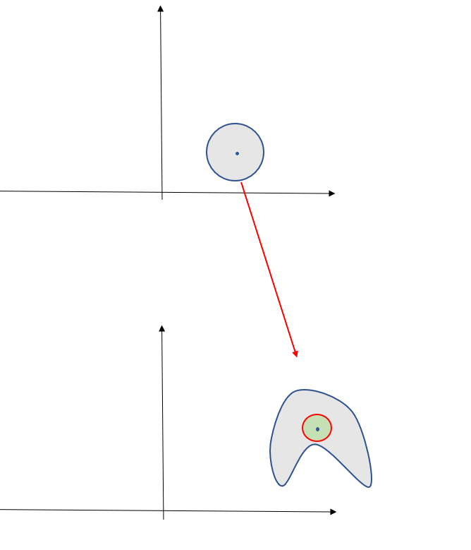
Our function P(z) = 2z was nice in that it exactly mapped the circle into a different circle. But we might have a more horrible polynomial, perhaps z⁷-3z² +1. A natural question then to ask is, if we see where a circle maps to, can we inscribe a circle? It doesn’t matter if the circle is really, really small. In the diagram above, the circle maps to some weird shape, but that doesn’t matter, because we can draw that small green circle with the red perimeter, which fits snugly inside the slightly odd shape.
Why is this helpful? Well, it turns out we can inscribe a small circle around P(w) provided the derivative is not 0 at w. We will also find out that the derivative can only be 0 at a finite number of points.
Previously, we looked at where a circle mapped to, but now we look at where the entire plane maps to. In particular, if we don’t have a point which maps to the origin, then for every line through the origin in the greenish blob below, we can consider the point on the line which is closest to the origin.
Let me take some time to explain the diagram below. Take a look at it first. The grey blob represents the complex plane. It goes on indefinitely in all directions. We then place a dot of green at every place a grey dot lands under the map P. The map P is kinda like a projectile firing points from one plane to another. We don’t know much about this green shape— in fact, even the diagram itself tacitly assumes some things, hence the need for formal proofs as well as pretty pictures! — but if there is no point which is sent to 0, then the origin is not shaded. It turns out there must be a region around 0+0i which nothing is sent to.
We then draw a purple line from the origin in the lower part of the diagram. We identify the closest point on that line to the origin, and we find which point was sent to it.
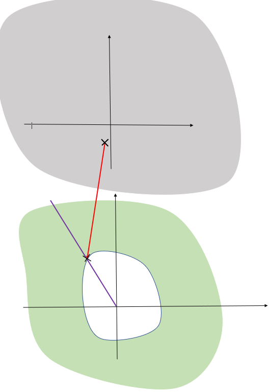
Here’s the trick. Suppose the point with the cross in the grey diagram is called w, and the one in the green diagram is P(w). Now suppose the gradient at w is non zero. We can then draw a small circle around w, and watch where it lands

In particular, the small grey area could contain a small circle, as per our previous discussion. But this is clearly a contradiction — the grey area, along with any other circle centred at P(w), clearly (visually) contains points on the purple line which are closer to the origin. But recall that, of all possible complex numbers z which were mapped such that they landed on the purple line, w was the one which landed closest. It is therefore a contradiction to find these points on the purple line closer to the origin which are in the image of the map P.
We can apply this to every single line through the origin, of which there are infinite. This argument only doesn’t apply when the derivative is 0, which occurs at most for a finite number of points. That still leaves an infinite number of lines where we can apply our argument, and we can still find our contradiction.
But now we hold our horses. This argument was pretty, and the diagrams were nice (well, sorta; I patched them together on microsoft word!). They give good intuition for the approach, but it is not yet a proof. For that, we need definitions which capture these geometric intuitions, and allow us to apply them rigorously to any polynomial.
1. Complex number basics
There’s several ways to approach what a complex number is. The ‘rigorous’ definition is probably only helpful to people who already know what a complex number is. So below is some visual understanding and intuition. If you already are comfortable with complex numbers, skip this section.
Visually a complex number z can be written as its ‘real’ and imaginary parts. The real part is written on the x axis of a graph, and the imaginary part is written on the y-axis. So z = x + iy.
Addition happens as you would expect: you add the ‘real parts’ and you add the ‘imaginary parts’.
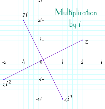
Multiplication can be visualised slightly differently: it corresponds to a rotation and a change in radius. Here, the square root of negative 1 makes perfect sense, as we have extended the definition of multiplication! The point i has angle 90 degrees, and length 1. So, when we multiply a point z by i, we rotate it by 90 degrees, and scale the radius by 1. Of course, scaling a radius by 1 leaves it the same. If we were to multiply z by 2i, then it would be rotated by 90 degrees, and stretched outwards by a factor of 2.
2. Some basics about polynomials
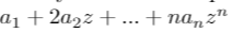
The complex derivative of the polynomial
is given by
While proving that the polynomial has a root is hard, bounding the number of roots is less hard. A polynomial of order n, i.e. one whose max power term is z^n, has at most n roots. That’s because we can factorise out the roots of the polynomial one by one

After factorising out the first n roots, it becomes apparent that any other number won’t evaluate to zero, as each term in the multiplication is non zero.
Polynomials are ‘continuous’ functions. As their derivative is a polynomial, its derivative is also continuous. But I will give more details on what, exactly, continuity means and what a complex derivative means, in the next section.
3. Analysis Preliminaries
3.1 What is a limit? Sequences, and convergence
Let’s understand what sequences and convergence are
A sequence of complex numbers is simply a list of complex numbers, where for any integer n, you are allowed to receive the nth number in the list.
One example of a sequence of complex numbers is:
0.9 + 0.9i, 0.99 + 0.99i, 0.999 + 0.999i, 0.9999 + 0.9999i, 0.99999 + 0.99999i, …
where the Nth number in the list has N nines following the zero for both real and complex part
We say this sequence ‘converges’ to 1 + 1i. Why? The first term is only 0.1 + 0.1i away from 1 + 1i, the second term is only 0.01+0.01i away from 1+1i, and the Nth term is 0.00…01 + 0.00…1i away from 1+1i, where there are N zeros preceding the 1. If we use Manhattan distance then the distances are (0.2, 0.02, 0.002, 0.0002, …) which clearly tends to 0. If we use euclidean distance, we find the distances are (sqrt(0.02), sqrt(0.002), sqrt(0.0002), …) which also tend to zero. In general, if a sequence converges with euclidean distance, it converges to the same place with Manhattan distance, and vice versa.
So a good definition for convergence to 1+1i is: for any maximum distance from the target you specify, I can find an N such that all terms after the Nth sequence are within that distance from 1+1i.
This definition makes sense. If you set the target to be 0.00234 away in both real and complex parts, then we observe that 0.001 is smaller than 0.00234, and that from the third term onwards:
- 1–0.999=0.001≤0.00234
- 1–0.9999=0.0001≤0.00234
- 1–0.99999=0.00001≤0.00234
- and so on
Clearly, whatever you set the maximum distance we are allowed from one, eventually we can find a 0.000000000000000000…00000001 which is smaller than that number, and use the same argument as above.
3.2 Continuous functions
A continuous function preserves limits. In the example above, a continuous function f would ensure that the sequence (f(0.9 + 0.9i), f(0.99 + 0.99i), f(0.999 + 0.999i), …) converges to f(1+1i). An alternative, but mathematically equivalent definition, is that if you set a target for closeness, be it 0.1, or 0.0000001, then whatever it is, you can find a distance d, within which all the points are within that closeness.
This is best illustrated by an example. Suppose you set the target of 0.001 at a point z. Then I find a distance, which might be 0.0142, where if |w-z|<0.0142, i.e. if w is contained in the circle centred at z and of radius 0.0142, then |f(w)-f(z)|<0.001.
The latter definition is captured in the famous epsilon-delta definition of continuity at a point z.

Or, for functions over the real variables, it is captured intuitively (although with some notable exceptions*) by a ‘line which can be drawn without taking your pen off the paper’.
*These sorts of functions are often called pathological by mathematicians. They often occur when a definition captures the essence of something, such as our intuitive notion of continuity, but it also turns out this definition includes several functions which do not align with our intuitions whatsoever.
3.3 Open and closed balls
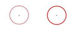
An important concept is the open and closed ball. The open ball centred at z with radius r is made by drawing a circle around z with a ‘dotted line’. This symbolises that it includes all points within the circle, but none on the boundary. The symbol we use to represent this is below

The closed ball is like the open ball, but it includes the boundary of the circle. The symbol we use for the closed ball of radius r centred at a point z_0 is below. (The z_0 will be used because we will have to find names for several complex numbers at once, and it is easier to give little numbers at the bottom than to find a new alphabet)

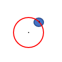
We say a point is in the interior of a set if we can find an open or closed ball surrounding the point fully contained in a set. So a closed ball has some points not on the interior, namely those points on its boundary. Any circle drawn around a point on the boundary will include some points not found within the circle. This can be seen below.
In contrast, every point in the open ball is on the interior, as the open ball doesn’t include any of the boundary point. No matter how close we are to the boundary, if we zoom in enough, there is enough room to fit in a small circle around our point.

In general a closed set is one which, like the closed ball, contains its boundary (technically speaking, contains all its limit points). An open set, like an open ball, does not contain its boundary, and you can always find a small open ball around a point where the open ball is fully contained in the set.
For instance, a rectangle with a ‘dotted line’ (a rectangle which doesn’t contain its boundary) is an open set, while a rectangle with a hard line (which does contain its boundary) is a closed set. For the closed rectangle, if you put a circle on the boundary, the circle always includes points from outside the set.


3.4 Image of a function
The image of a function is a set containing all points which the function can send something to. For example, if a company had a function which took in a flight number as an input, and destination country as output, the image is the set of all countries the company flies to. In our case, it is all points v such that there is some z where P(z) = v. (all countries v such that there exists some flight number such that P(flight number) = v)
We can consider the image of a smaller subset of the complex plane. For instance, suppose we wanted to consider all the points v such that there exists a z in the circle B such that P(z) = v (woah that’s a mouthful). We would then call this the image of B under P.
A worked example. Consider the function P(z) = 2z. The image of P is then the whole complex plane: given any point v, there exists a point z - in this case, v/2 itself - such that P(z) = v. P(v/2) = 2v/2 = v. If B was all points with radius less than or equal to 1, i.e. points in a closed ball with radius 1, centred at the origin, then the image of B under P would be the circle of points with radius 2. For instance, P(1+0i) = 2+0i.
4 Representations of a complex function and the Cauchy-Riemann Equations
There are several ways to represent a continuous, and differentiable, complex function.
We often just write f(z). For instance, f(z) = z + z³ + 1+2i is a complex function. We can also split it into real and imaginary parts. In that case we write f(z) = f(x+iy) = u(x,y) + iv(x,y). It turns out that, for a complex function is continuous only when u(x,y) and v(x,y) are continuous.
Another slightly odd thing about complex numbers is how to differentiate them. We want the following expression to converge as h tends to 0

However, as we are dealing with complex functions (i.e. a function which takes a complex number as an input, and a complex number as an output), the conditions are a little stronger than for real functions. That’s because the complex numbers are a plane: a 2-dimensional object. So our limit can come from any direction: left, right, up, down, spiral, you name it. Whereas in normal calculus, we can only approach a number, say 3, in a one-dimensional manner (i.e. from the left, such as 2.9, 2.99, 2.999, 2.9999, and from the right, such as 3.1, 3.01, 3.0001, 3.00001, …).
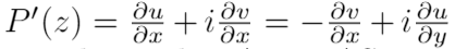
The conditions for a complex function to be differentiable can be captured in two very simple, but fundamental, equations.
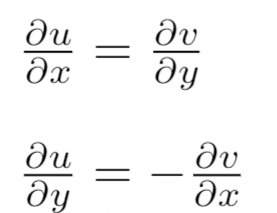
These two equations capture that we want the derivative to be the same whichever direction we approach from.
There’s many a wonderful theorem which follows from this simple assumption, which actually give another way of proving the fundamental theorem of algebra. Our proof is more elementary — it won’t rely on the most powerful theorems of complex analysis, at the trade off of being more complicated.
The Proof
Part I: at most N-1 points of a polynomial are not on the interior.
In the first part of the proof, we establish that all but a finite number of points of the polynomial are not on the interior.
Part IA.
We learned that the number of roots the derivative has is at most N-1. The idea is to leverage this, by looking at closed and open balls where the derivative is non-zero for every point in the ball.
Exercise: draw the 2D plane. Draw three points. Given a fourth point, can you draw a circle around it which doesn’t contain those three points? Likewise, given a finite number of points where the derivative is zero, and every other point we can draw a circle small enough such that it doesn't include a point where the derivative is zero.
We take a point z_0. We want to show that P(z_0) is on the interior of the image of P. (where P is our polynomial function). This means that we want to be able to draw a small ball around wherever z_0 landed after being evaluated by P, and for every point in that ball, there exists a point z such that P(z) evaluates to that point.
An example of where this isn’t possible is the function T(z), which sends every point in the complex plane to 1+0i. Then, any circle containing 1 also contains points which are not 1. If the radius of the circle was 0.05, then it would include 0.99+0i. But there is no point z such that T(z) = 0.99, as T sends all points to 1.
[this property of being in the 'interior' might be a slightly confusing property to be investigating at first. It will pay dividends]
Part IB. Interior points are preserved under multiplication
Given our polynomial P, suppose we are at a point w, and have a derivative at that point P’(w) = a+ib. (Note the apostrophe to denote the derivative). If the derivative is non-zero, then we can consider a different polynomial, P(z)/(a+ib). This new polynomial behaves very similarly to the previous one, but its derivative at w is 1+0i. (That’s because if we scale a function by a constant, the derivative gets scaled by the same constant).
This will be a very handy simplification for later in the proof. But we need to prove that w is on the interior of P(z) if, and only if, w is on the interior of P(z)/(a+ib). A way of visualising this is that complex multiplication scales the radius and rotates the angle. So we we multiply the ‘ball’ surrounding P(w)/(a+ib) by (a+ib) this rotates and stretches every point on the ball, resulting in a new ball surrounding P(w).
Part IC. A useful inequality when P’(w) = 1+0i
Here we show a helpful inequality we can use when the derivative of P at w is 1+0i, i.e. P’(w) = 1+0i. We will show that in a circle containing w, that if w and v are some distance, L, apart in this circle, then P(w) and P(v) are at least 0.8L apart, when measuring distance with Manhattan distance.
For this inequality, we will represent P(z) as u(x,y) + iv(x,y), which is one of the methods of expressing a complex function discussed previously.
First, we use the triangle inequality

Second, recall the Cauchy-Riemann equations.
Moreover, both these partial derivatives are continuous.
(Note to maths nerds) it is ok to assume this, because for a polynomial both u(x,y) and v(x,y) are just polynomials in two variables, so the apparatus normally used to prove continuity of the partial derivatives is not required. In general, proving that the partial derivatives are continuous is not so easy.
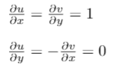
In this case, we are assuming that P’(w) = 1+0i. So we update our equations to include this information
Using continuity of these derivatives, we can find a circle in which they stay within these bounds. Remember this inequality for later!!!
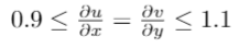

It is worth noting that there is nothing special about the numbers 0.1, -0.1, 0.9, 1.1. There are many numbers I could have picked which give an equally useful inequality.
Next we use our our knowledge of calculus in one variable to make it useful here.
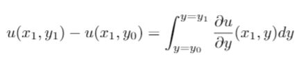
For instance, if x = 0.2, then u(0.2, y) is a function in one variable, and the normal rules of one variable calculus applies. Basically, we are finding a way to carry across our knowledge of one variable calculus into this new setting.
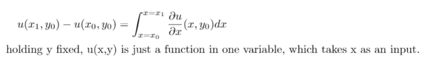
We use a similar idea again:
Combining these two equations we get:


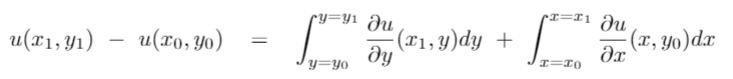
The integral with respect to x is always greater than 0.9|x_1 — x_0| because its length is |x_1 — x_0| and the height of the function is always greater than 0.9. [Recall the inequality I asked you to remember for later?). The integral with respect to y is never more negative than -0.1|y_1 — y_0| because its height is never lower than -0.1, and its width is |y_1 — y_0|

As a general rule in mathematics, you can’t overuse a good idea. Applying the same logic as previously we get a similar looking equation for v(x,y)
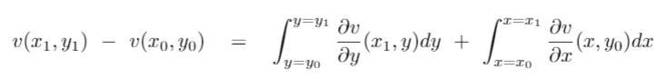
Using near identical reasoning as we did for u(x,y), we get

Combining the two, we can conclude that

Part ID
Some parts of this section are moderately technical. Try to get a feel for the arguments without necessarily getting to bogged down in them. Most of this is the technical implementation of the overview given in the section ‘0. Gameplan’
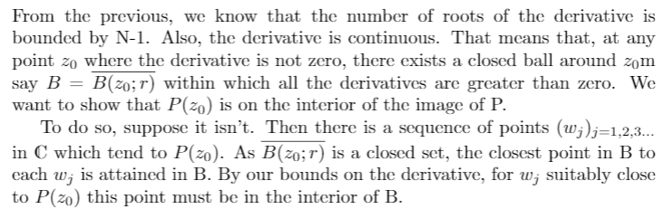
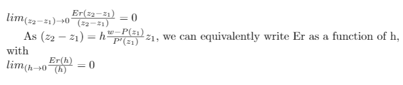
We use now proof by contradiction to conclude Part I of the proof. Recall that our point w has the property that P’(w) is not 0+0i, and we want to show that it is on the interior. Further recall, that showing P’(w) is on the interior when P’(w) = 1+ 0i is sufficient to prove the more general case of when P’(w) can be anything except 0 + 0i
As the derivative is not zero, and is continuous, we choose a small circle around z_0 to be small enough so that the derivative is bounded away from 0. We call this circle B.
Suppose that our point P(z_0) is not on the interior of the image of B under the function P. Then, whenever we draw a circle around P(z_0), there is some point not in the image of P but is in that circle.
Side note. If this terminology makes you uncomfortable, take another look at the Preliminary Section on Images of functions.
This is seen visually below. If the circle surrounding the point is not completely contained in the image of P, then we can find at least one point which is both in the circle and not in the image of P. We can do this for a circle with arbitrarily small radius, thus allowing us to construct a sequence of points not in the image of P, which get ‘arbitrarily close to’ P(z_0).
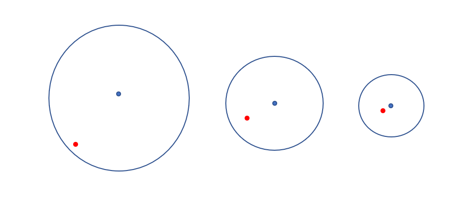
Making the radius of the circle we draw successively small, we conclude there is a sequence of points which converge to P(z_0) but are not in the image of of P with domain being a small circle around z_0.
These red dots (see picture) cannot exist in isolation. The image of B is a ‘closed set’, which means it contains its limit points. Thus, if there were points in the image of B arbitrarily close to the red dot, the red dot would be a limit point of B and thus included in B. Thus, the red dot is itself surrounded by an open ball which contains no points in the image of B.
Behind the scenes, we have to mess about with the domain being a compact set -closed and bounded -, the function being continuous and then we can guarantee that the image of B is compact.In the argument below, existence of some of the points also requires using compactness and continuity arguments.
For each of the red dots, we can consider the point in the image of B closest to it. Let’s call this P(z_1). Using our inequality from Ic, provided P(z_1) is close enough to P(w), then we know for sure that z_1 is not on the boundary of B — i.e. on the edge of the circle. In particular, z_1 is on the interior of B.
Intuitively: we showed that if P(z) is 'close' to P(w), then z is 'close' to w. Provided P(z) is 'close enough' to P(w) relative to the distance between wand the boundary of B, then we can be sure that z is not on the boundary of the ball B.
Written up nicely in LaTeX:
Part 1E:
This section is also quite technical.
Some intuition. As z_1 is in the interior of the ball B, we can take a small step in any direction and remain in the ball B. We can use the derivative to approximate P with a linear function. We can then roughly calculate where this step will land us, with a small error term. By choosing our direction right, and our step small enough, the error term is not large enough to stop us moving closer to the red dot.
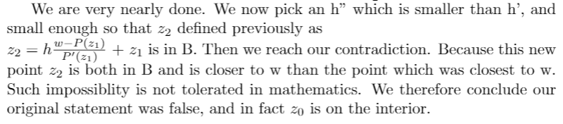
Take our point z_1. It was the closest point in the image of B to one of the red dots. We want to prove there is a closer point, and thus arrive at a contradiction.
We define z_2 as below.
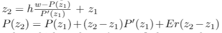
In the above, h will be some small value which we haven’t specified yet, and second expression is a linear approximation. This linear approximation is very good locally, as it is defined using the derivative P’(z_1). In particular, Er is the error term from the linear approximation. The error term decreases very quickly:
The above is almost a definition of the derivative: that we can take a linear approximation, and the error to the linear approximation disappears faster than our distance from z_1.
Now, we do some fairly simple, but messy, algebra (just manipulating the definitions above). Take my word for it if you’re somewhat exhausted at this point :)
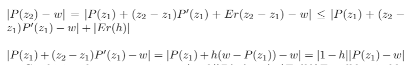
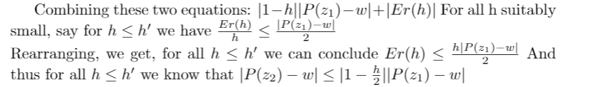
I repeat the intuition from earlier: As z_1 is in the interior of the ball B, we can take a small step in any direction and remain in the ball B. Thanks to the derivative as an approximation, we can roughly calculate where this step will land us, with a small error term. By choosing our direction right, and our step small enough, the error term is not large enough to stop us moving closer to the red dot.
Part II: Concluding the argument
The idea for concluding the proof is that, for every straight line through the origin, we can examine the point on that line which is closest to 0+0i.* All but N-1 of them we know to be on the interior. As there are an infinite number of straight lines which pass through the origin, even after discarding these N-1 points that leaves us with an infinite number of points* which are both (1) the closest point on that line in the image of P to the origin, and (2) on the interior of the image of P. Being on the interior means that we can draw a small circle around them which is contained in the image of P. But this small circle contains points on the line which are closer to the origin — a contradiction.
Thus we may conclude that our polynomial has a root.
*proving these ‘rigorously’ requires a little bit more fiddliness, which we omit here, as it is more tedious than it is enlightening.
A final word
If you have made it this far, thank you and well done :) I hope you enjoyed. The argument I have presented here is not every single detail, but it is most of the detail, and I think any more would be unreadable (or, more unreadable!). You can follow me on twitter, where I am ethan_the_mathmo, link here. Let me know comments/thoughts/suggestions/requests/you-name-it, down below.
Thank you to Bartek Pierzchała for reading through the proof, and helping with readability.


