All About Root Systems

This is a gentle introduction to an important concept in combinatorics that plays a major role in algebra and geometry — root systems. Roots are just vectors in a real vector space with some special properties. A root system is a collection of roots. The special properties have to do with reflections and whether the roots generate a lattice. In what follows I’ll try to introduce root systems using a series of diagrams that I produced using TikZ (a graphics package for LaTeX) and describe Coxeter-Dynkin diagrams (which I plot using dynkin-diagrams, another LaTeX package). I hope these figures make it easy to get started with root systems and appreciate their structure in higher dimensions.

One Dimension

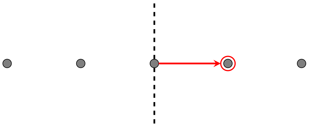
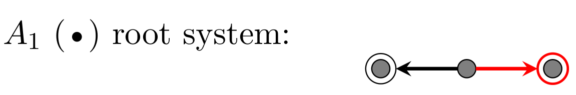
Let’s begin with the one-dimensional root system, the A1 root system. First take a simple root, shown here as a red vector.

Each root system begins with a set of simple roots. While the full set of roots span the vector space that contains them, the simple roots form a basis for that vector space. So we need exactly n simple roots to construct a root system in ndimensions. In one dimension, we only have one simple root. Every root defines a plane perpendicular to it, which we will call a reflection plane.

The plane defines a reflection, and so each root defines a root reflection — a reflection through the plane perpendicular to that root. In this case, there is only one root and it is reflected through the plane orthogonal to it. This is typical behaviour — the reflection defined by each root sends it to its opposite root.

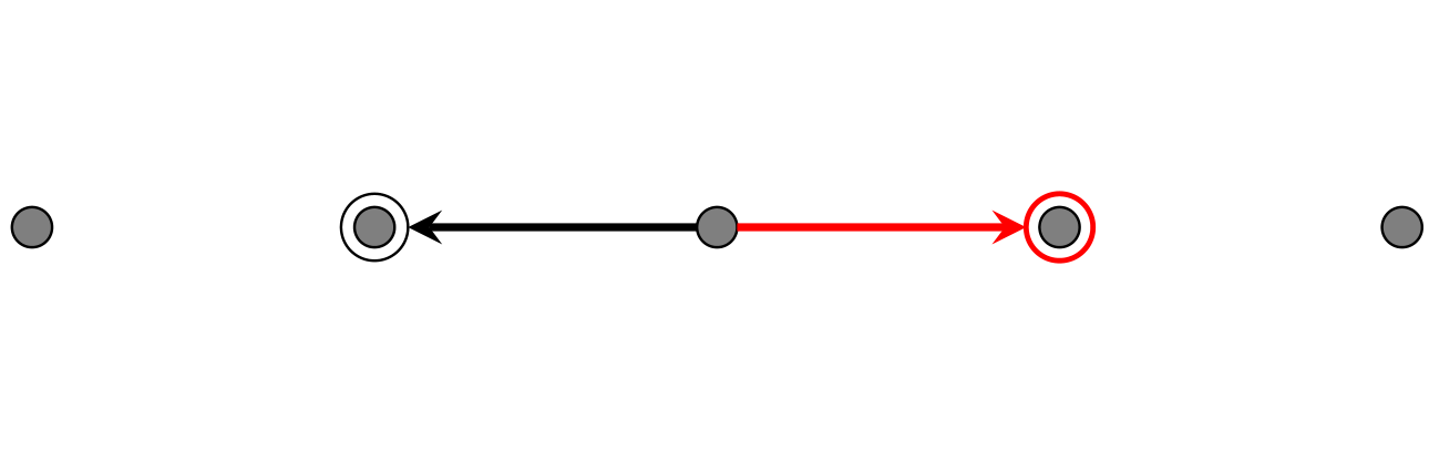
That’s it! We have constructed the A1 root system — just two opposite vectors of equal length. Why is this a root system? Because the reflections defined by each root (both the red and the black vector) send each root to another root. Both roots here define the same reflection plane, and the reflection simply swaps them. We say that these vectors are closed under root reflection, meaning that each vector defines a reflection symmetry of the set of vectors. Also, you may have noticed the dots on the diagrams. Every root system has a corresponding root lattice. We construct the root lattice by taking all the sums and differences of root vectors. In the case of the A1 root system, the lattice is an infinite set points at equal distances along a line. In fact, the A1 root lattice looks like a scaled version of the integers on the real number line.

Two Dimensions

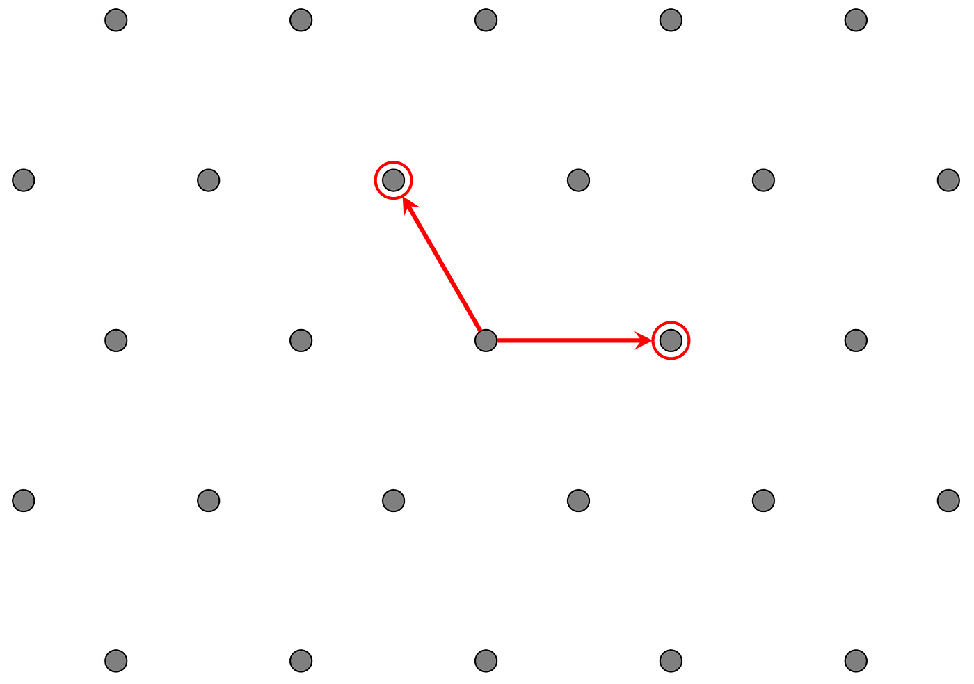
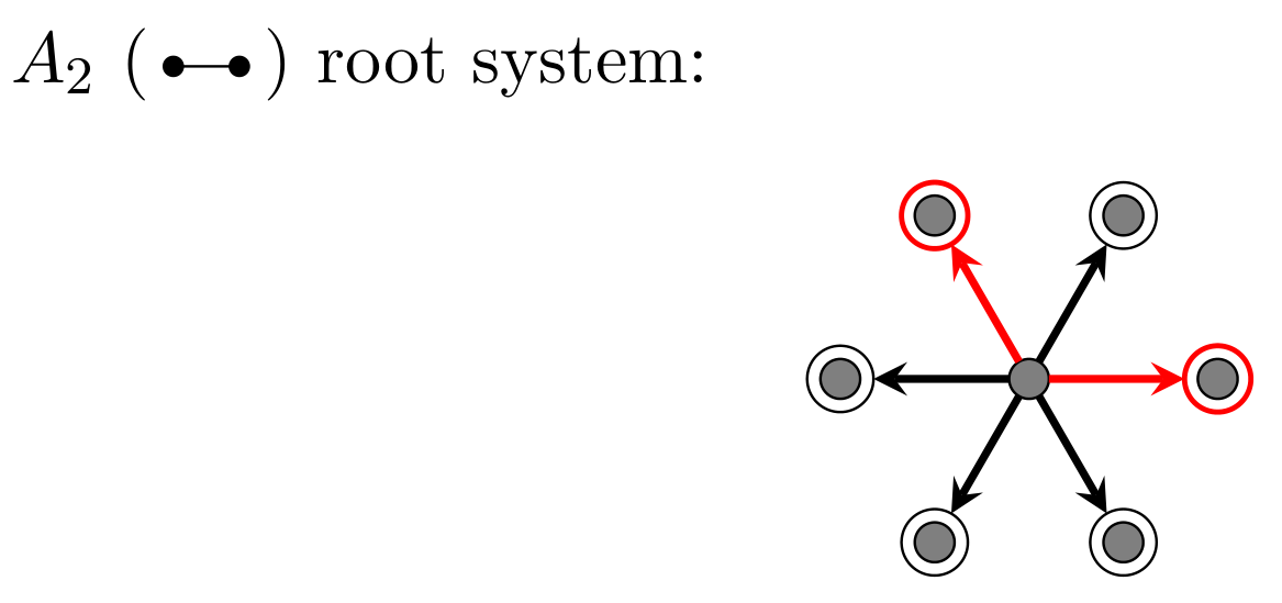
Let’s move up to two dimensions. Now we are working in the real plane and therefore we need two simple roots to get started. There are a few choices available, since there are more than one root systems in two dimensions. Perhaps the most important example is the A2 root system, which begins with a pair of simple roots at 120 degrees. We always choose simple roots so that each pair is either orthogonal or at an obtuse angle.

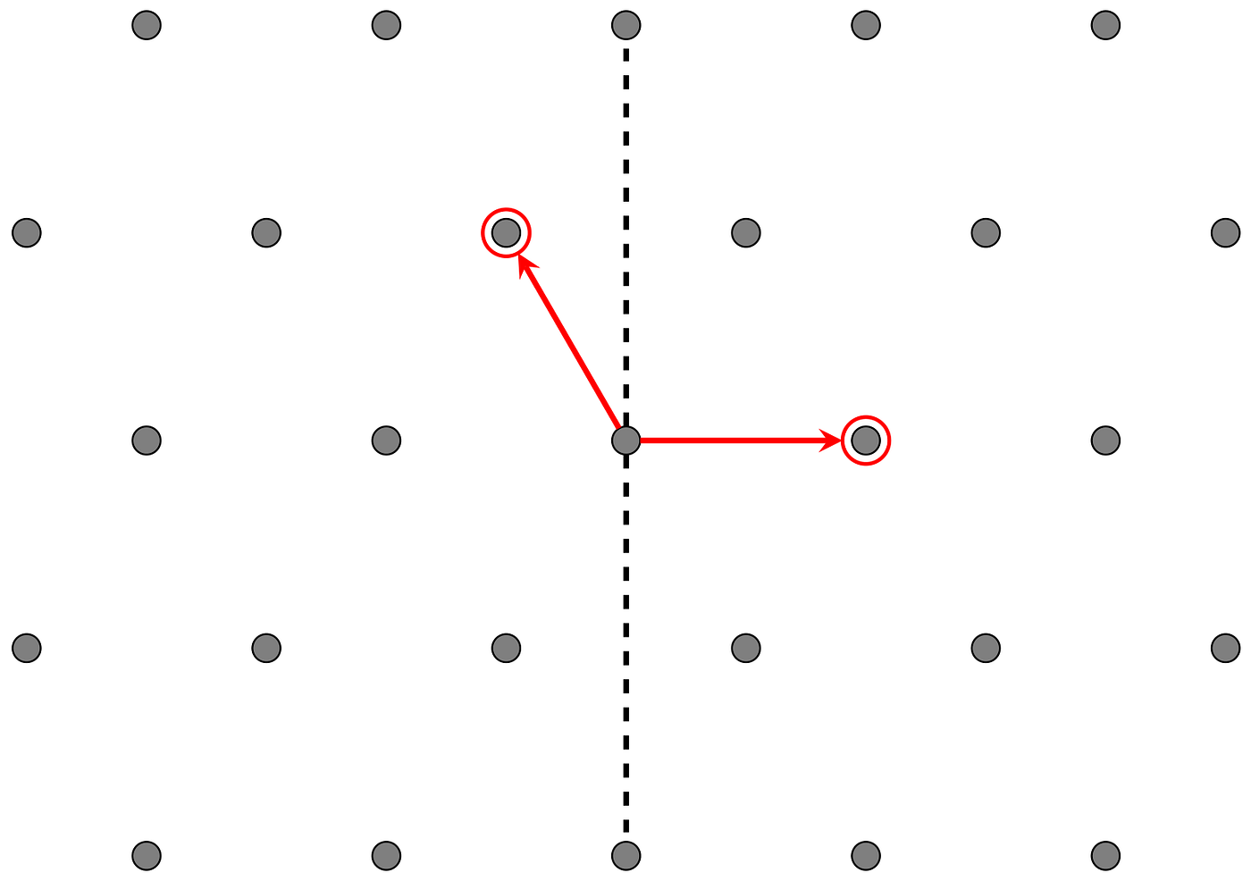
As before, we can define a reflection plane orthogonal to each simple root.

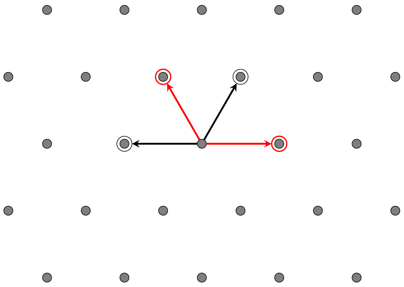
In this case, the reflection gives us two more roots.

To obtain even more roots we define the reflection plane orthogonal to the second simple root.

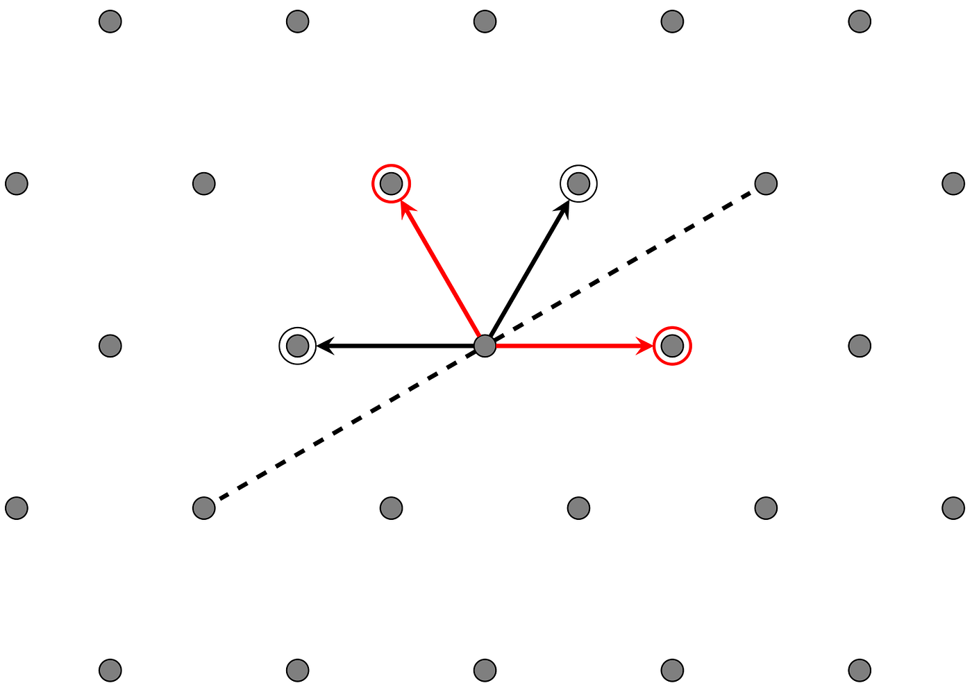
This gives us our last two roots.

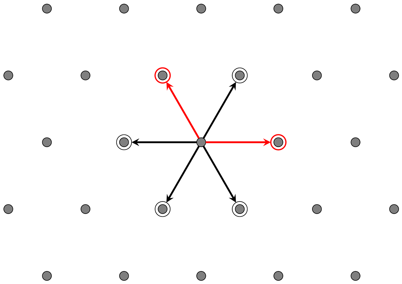
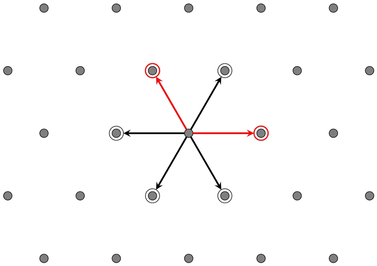
If you look closely you’ll notice that no matter which of the six roots we choose, the corresponding reflection always sends roots to roots. This completes our construction of the A2 root system.

Notice that the root lattice of A2 is the familiar honeycomb pattern. Also notice that although this lattice is spanned by the six roots, we only really need to take sums and differences of the two (red) simple roots to get to any point on the lattice. Also, just as we could treat the A1 lattice as the set of integers on a scaled real number line, we can also treat the A2 lattice as a set of points on a scaled complex plane. It turns out that just as the integers in the real numbers are closed under addition and multiplication, the A2 lattice points in the complex plane are also closed under addition and multiplication. This system of integers in the complex numbers is known as the Eisenstein integers.

Higher Dimensions

To handle root systems in higher dimensions, we must use new tools since we can’t plot all the roots in the way that I’ve done above. Instead, we focus on the simple roots (the red vectors in my diagrams). The best tools for this job are the Coxeter-Dynkin diagrams.

In a Coxeter-Dynkin diagram, each node (or vertex) represents a simple root. When two simple roots form an angle of 120 degrees, we place an edge between them. If they form an angle of 90 degrees, we do not place an edge between them. Once we have defined the simple roots of a root system, we can recover the full set of roots using reflections in the same way that we did above.

For example, the A1 root system has just one simple root and the Coxeter-Dynkin diagram is just a single node.

The A2 root system has two simple roots at 120 degrees. So the Coxeter-Dynkin diagram is two nodes connected by an edge.

To recover the full root system we begin with the simple roots given by the Coxeter-Dynkin diagram and carry out root reflections until we do not obtain any new roots.

We say that a root system is indecomposable when there is no way to partition the roots into two mutually orthogonal sets. The indecomposable root systems are fully classified. We can list them all using this short list of Coxeter-Dynkin diagrams:

In this classification we have four infinite families and five exceptions. You may notice that some of these diagrams have double or triple edges with arrows. These signify new cases that emerge when we begin with simple roots of different lengths. When we do, the arrow points from the long root to the short root. Here are the rules:

• In the case of the double edge, one root has a length-squared that is twice the length-squared of the other. This corresponds to an angle of 135 degrees.
• In the case of a triple edge, one root has a length-squared that is three times greater than the other. This corresponds to an angle of 150 degrees.

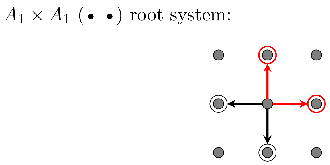
In one and two dimensions, the full list of root systems is given by the following Coxeter-Dynkin diagrams:

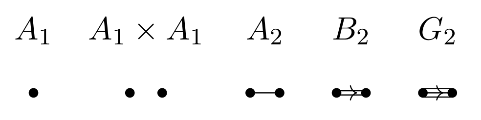
The A1 x A1 case begins with two orthogonal simple roots and gives us a square grid lattice.

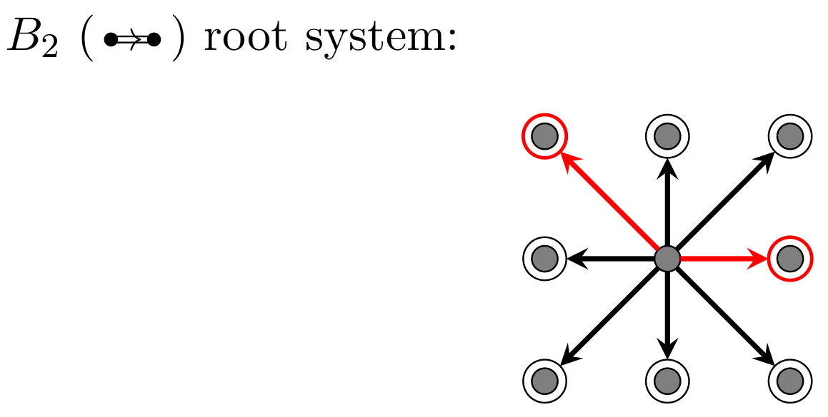
The B2 case has the same lattice but begins with two simple roots at 145 degrees instead. This means that B2 has an A1 x A1 subsystem of roots.

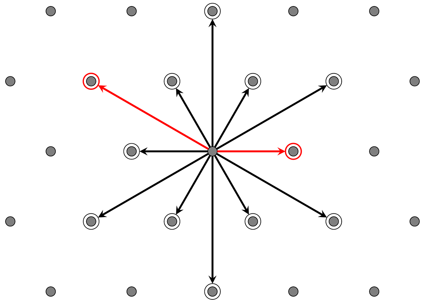
Finally, the G2 case shares the same lattice as A2 but begins with two simple roots at 150 degrees. This means that G2 has A2 as a subsystem of roots.

Simply-Laced Diagrams and the “A, D, E” Pattern

The root systems of types A, D, and E are special in a number of ways. The key is that they have Coxeter-Dynkin diagrams that lack any double or triple edges. When a Coxeter-Dynkin diagram has only single edges, we call it a simply-laced diagram. A simply-laced diagram describes a set of simple roots where each pair is either orthogonal or at 120 degrees.

The A, D, E root systems turn out to be related to a structure known as the star-closed line systems, which are describe by Cameron and van Lint in their book “Designs, Graphs, Codes and their Links.” A line system is a set of lines where each pair is either orthogonal or forms an angle of 60 degrees. A star is a set of three lines in a plane, each pair at 60 degrees. To visualize a star, just imagine the three lines through the pairs of opposite A2 roots.

We can recover a star from any two of its lines, and a star-closed line system is a system of lines in which we supply any missing third lines of the star defined by each non-orthogonal pair. Finally, a star-closed line system is indecomposablewhen there is no partition of the lines into mutually orthogonal sets.

Remarkably, the indecomposable star-closed line systems are precisely the lines defined by the pairs of opposite roots in root systems of types A, D, and E. So the question of constructing all root systems of types A, D, E is equivalent to the question of finding all star-closed line systems.

I am really struck by the fact that root systems properties are generally reducible to properties about star-closed line systems and their symmetries. In many ways line systems are simpler to grasp, since each pair of opposite roots define a line and when we work with lines we don’t have to worry about whether the angle between them is obtuse or acute. In fact, in the context of star-closed line systems, all that matters is whether two lines are orthogonal or not. It doesn’t get much easier than that.

There’s much more. Every root lattice can be constructed from the short roots alone. This means that although there are root systems of types A, B, C, D, E, F, G, there are only root lattices of types A, D, E (this is discussed in Conway and Sloane’s book, “Sphere Packing, Lattices, and Groups”). The relation between G2 and A2 is a helpful example here. Notice that the lattice of the G2 root system is just the honeycomb lattice of the A2 system. The long roots of the G2 root system are themselves A2 lattice points.

What Next?

As far as applications go, Lie and Jordan structures are closely related to what I’ll describe as continuous symmetries, analogous to rotations in higher dimensions. But these symmetries are strongly constrained by the classification of these innocent looking vectors known as roots. Indeed, up to isomorphism there is a unique semi-simple Lie algebra for each root system, and a unique root system for each semi-simple Lie algebra. This suggests that getting a feel for root systems can pay off in unexpected ways. The available symmetries in nature (or in the Platonic realm if you prefer) are governed by root systems. This surprising fact keeps me interested and sometimes vexed as I try to visualize these creatures in their higher-dimensional natural habitat.