In this article we explore how the principle of relativity may apply to curvilinear movements.

Our aim will be to achieve a transformation analogous to that obtained by Einstein on his paper On the electrodynamics of moving bodies [1], the Lorentz Transformation, but referred to systems on rotational movement respect each other.

For that sake we will first apply Galileo’s viewpoint of relativity and then follow Einstein’s postulates. Therefore, we will figure out an Angular Galilean Transformation, and then add the postulate of a maximal angular speed. We will find out that an extension of Eintein’s apparatus will be needed, in order to have light as the measuring tool for times and curved paths. Finally we will propose an Angular Lorentz Transformation, and derive some results.

The Angular Galilean Transformation

Galileo noticed that, when two objects move with constant linear speed respectively, it is either one or the other that is actually moving at that speed respect to one another, but in opposite directions. He accurately expressed his principle through a set of equations known as the Galilean Transformation[2].

The same observation can be made with objetcs moving with constant angular speed respect each other. The best evidence is the apparent movement of celestial bodies around the Earth. Thus we may write a corresponding set of equations:

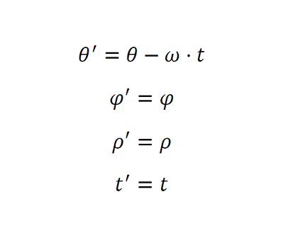
Note that this set of equations is mathematically identical to the aforementioned Galilean Transformation, only acquiring another meaning when agreed a specific physical context to the variables. This is, ω will mean some angular speed, θ will mean some angular displacement, and so on.

The Angular Speed Limit

Since the speed of light through vacuum is the actual speed limit in our universe, and given we can relate angular and linear speeds through the following identity,

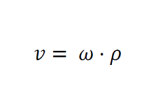
then we may expect the existence of an angular speed limit, anytime the radius to consider is always a finite quantity, since it must be any of these 3 quantities: an infinitesimal quantity tending to 0, some determined quantity or the highest possible value, this is, the ending edge of the universe.

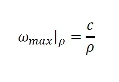
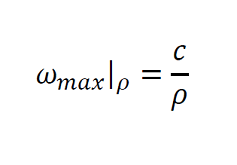
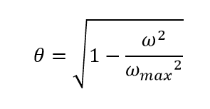
Considering a given radius ρ, let this angular speed limit be:

On Pursuing an Angular Lorentz Transformation

Once we assume a law of an angular speed limit, following Einstein’s line of thoughts, we can no more sum up speeds indefinitely using the Galilean Transformation, since this would eventually break the law. We therefore need to come up with a new transformation which doesn’t restrict the number of sums, the result of which always being below the limit.

We feel tempted to use the linear Lorentz Transformation straightforward as we did with the Galilean, but we wouldn’t have a pure justification for that proceeding. We shall then revisit Einstein’s steps in order to see how they fit for the angular case.

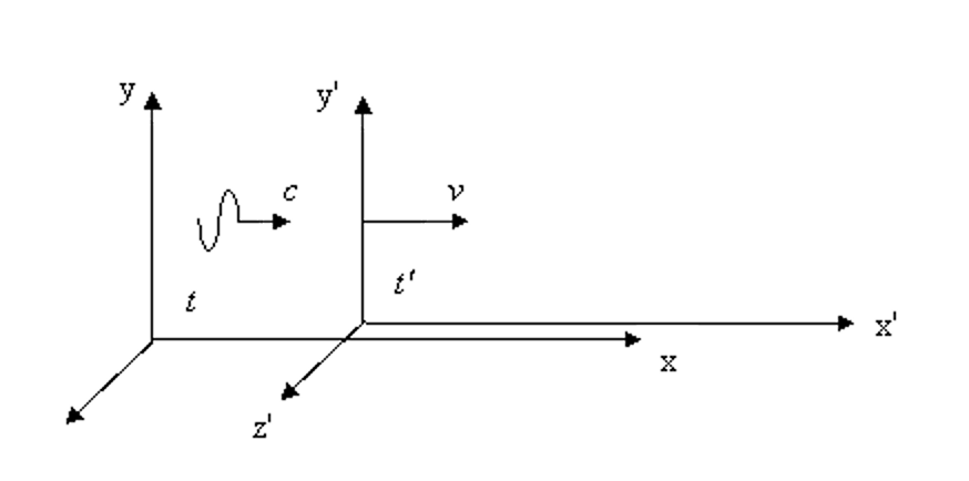
On deducting the Lorentz Transformation, he established 2 frames of reference, a stationary system K at rest, and a system moving in uniform translatory motion with respect to it, K’. A light ray would be emmited from the former to the latter, where it would be reflected backwards to the origin again. This works perfectly for a straight path, and thus he could deduct transformations for rectilinear lengths, but won’t work for angular measures, since light rays follow straight paths.

The following question arises: how can we use light to measure angles? The answer resides in the mixture of these two ideas:

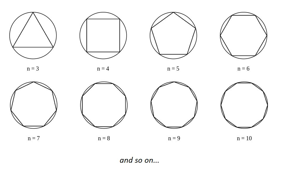
1. Instead of the path between 2 given points, we can use any arbitrary number of points, once they are positioned over an imaginary circumference traced between the first and last, and an implicit center of the circle. For this arrangement to work, we just have to build partial reflections within the inner points (those between the edges) and a total reflection at the ending point (just the same as in Einstein’s set up).
2. Increase masively the number of points and apply the same reasoning as Archimedes did for approaching the value of π.

In this manner we achieve our aim of having light travel straight segments while at the same time tracing a curvilinear path overall.

The Angular Lorentz Transformation

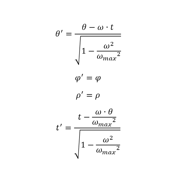
Now we are in disposition of following Einstein’s steps for inferring the angular transformations and so the equations obtained are completely analogous to those found by him, but for angular variables:

An Extended Case of The Lorentz Transformation

Note that, in order to embrace all this reasoning, we have had to implicitly account for the existence of a radius ρ, located at the center of the imaginary circumference described by the moving system K’.

Actually, with this in mind, the Lorentz Transformation is no other than a special case of the proposed Angular Transformation, when ρ → ∞ .

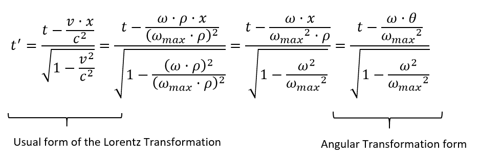
In fact, we can seamlessly switch between both transformations applying the following elemental concepts.

1. When multiplying the angle θ (or θ’) by the radius ρ, we are measuring the length of the arc, which is a linear distance, therefore finally obtaining the usual form of the Lorentz Transformation.

2. As per the relation between linear and angular speeds above exposed, we can easily switch the time coordinate of the transformation to the angular form:

Radius Contraction and Density Increase

Now if we follow the guideline given by Einstein for measuring lengths (angular in our case), initially we find that a curved rod of θ’ = 1 radian, comoving with K’,will be shorter if measured from K, the relation being:

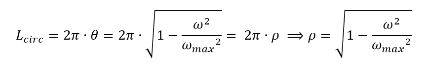
Since we need 2π of those rods lied together in order to complete a circumference, it is clear that this will be a shorter one when viewed from the stationary reference frame. And therefore also its radius:

Now it is obvious that if the radius is shortened, so does the area of the circle inscribed, and by the law of conservation of masses, then the density of the matter inside contained increases.

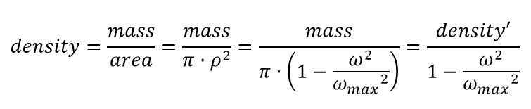
Therefore systems describing curved paths are perceived smaller and compact from the point of view of a stationary observer.

Note: This content belongs entirely to the author’s thoughts. Please don’t use it as academic content.

References

[1] On the electrodynamics of moving bodies, Annalen der Physik, A. Einstein.

[2] Galilean Transformation, G. Galilei.