A No-Nonsense Introduction to the Physics of the Big Bang

An Introduction to Cosmology and the Birth of the Universe

Cosmology is the study of the dynamical behavior of the entire universe. Modern cosmology is currently dominated by the Big Bang theory, which attempts to put together in one framework (or model) astronomy and elementary particle physics. One example is the ΛCDM model (or Lambda cold dark matter model) which will be discussed in more detail below.

As its name says, this model includes many types of matter and energy such as:

• dark energy (represented here by the cosmological constant Λ)
• the postulated cold dark matter (abbreviated CDM)
• ordinary matter.

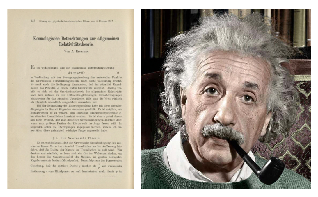
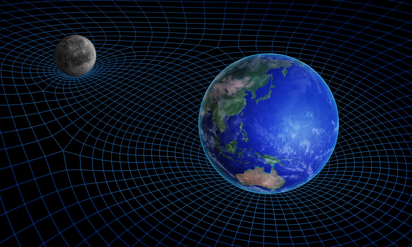
Modern cosmology was born when Einstein published his paper “Cosmological Considerations on the General Theory of Relativity” which applied his theory of gravity to the whole universe.

Standard Model of Cosmology

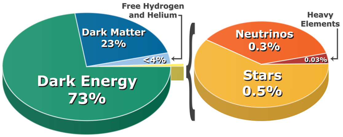
Our current standard model of cosmology today is the ΛCDM. In the ΛCDM model, the total energy of the universe is divided into three components: matter, dark matter, and dark energy. This division is based on data from the WMAP (Wilkinson Microwave Anisotropy Probe), “a NASA explorer mission (an uncrewed spacecraft) that was launched in June 2001 to make fundamental measurements of cosmology” quoting NASA’s website.

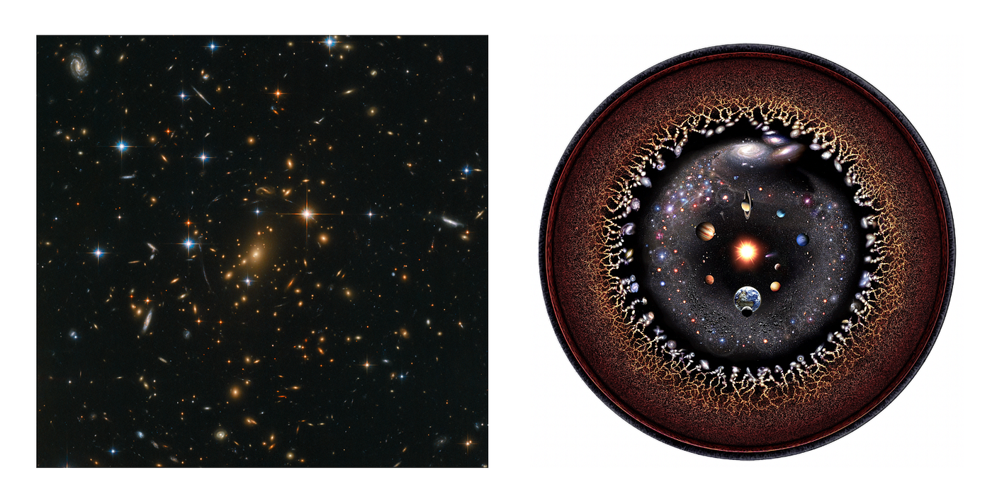
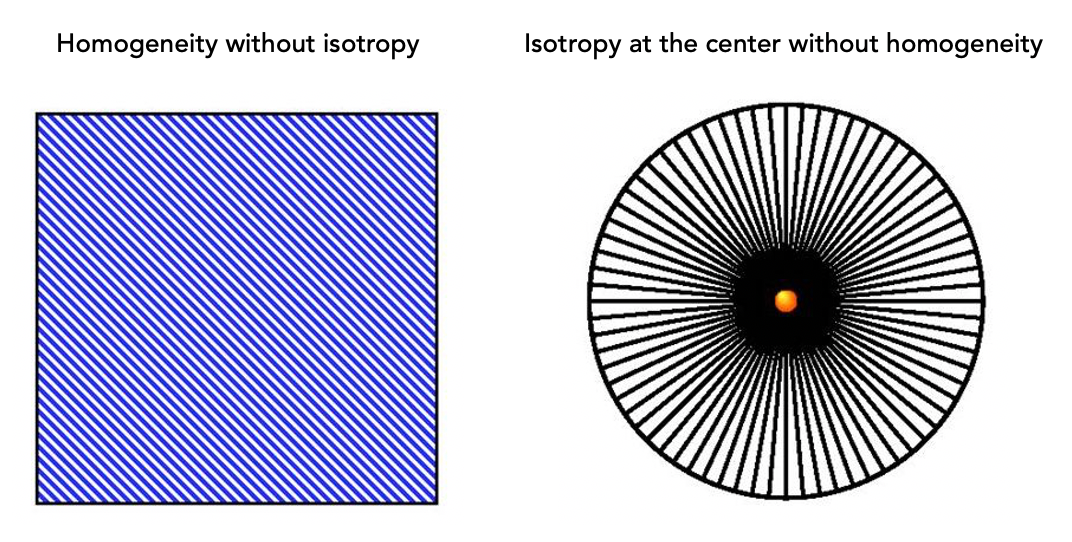
Homogeneity and Isotropy

If we consider regions of the universe that are sufficiently large (for example, galaxy clusters), the geometry of the universe is nearly homogeneous and isotropic (these hypotheses constitute the so-called cosmological principle).

• Homogeneity means having the same properties at every point
• Isotropy means uniformity in all directions.

The Metric of the Universe

Consider the metric tensor g, which “captures all the geometric and causal structure of spacetime, [and it is] used to define notions such as time, distance, volume, curvature, angle, and separation of the future and the past.” Homogeneity means that g does not change at different points of the universe (recall that this is valid only at very large scales). Isotropy means that g is spherically symmetric about any point in spacetime. A consequence of these two properties is that the curvature K of the spatial part of the metric g is constant.

Now consider an n-dimensional Euclidean space.

According to Shur’s theorem, if all points in a neighborhood of a given point are isotropic, and the dimension of the space is equal or larger than 3, the curvature K is constant throughout the whole neighborhood.

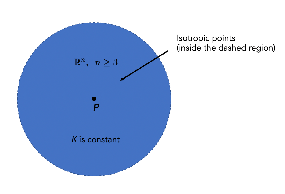
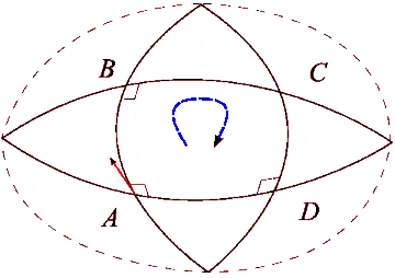
In our model of the universe, the curvature K is constant everywhere since we are supposing that the universe is globally isotropic. In each isotropic point the Riemann curvature tensor (see the animation below) can be written as:

A nonzero Riemann curvature tensor is a consequence of the fact that after the vector is parallel transported back to its starting point, it becomes a different vector.

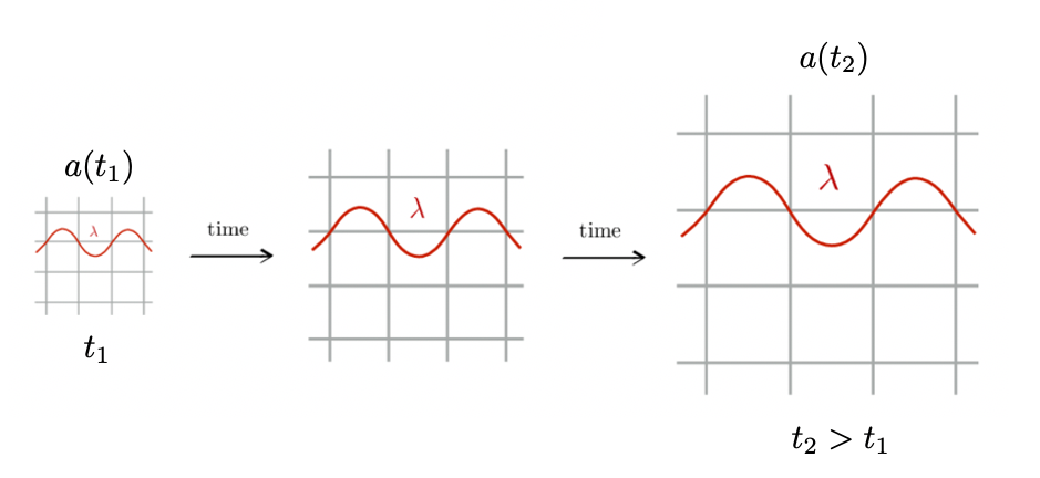
Note that our universe is globally symmetric in space only, not in time (as we know from observation, that the universe is expanding). The line element than can be written as:

where R(t) indicates the time evolution of the spatial slices of the universe and tells us how big these slices are at time t. The angular spatial part of the line element can be written as:

The tensor γ is homogeneous and isotropic. The u-coordinates are coordinates on the spatial slice and are called comoving coordinates. Observers at constant u are comoving and they see the universe as isotropic.

A Very Short Physical Interlude

It is clear that the points in spacetime and spacetime coordinates are two completely different concepts. As observed in one of my previous articles coordinates are merely labels and their choice does not change the laws of physics. When a(t) changes, physical points also change position but their distance in the comoving coordinate system stays the same.

The corresponding Ricci tensor then reads:

Our model of the universe is maximally symmetric. Maximal symmetry implies spherical symmetry. From the discussion of the Schwarzschild black hole in Carroll, we find that a spherically symmetric spatial metric can be written as:

where r is a radial coordinate and:

A Brief Mathematical Interlude

To continue, we will need the concept of tensors (see Dirac). I shall not give here a detailed explanation of the properties of tensors since we will not need it. The following article discusses in reasonable detail what tensors are (in case you are curious).

Quantum Gravity, Timelessness and Complex NumbersIs The Wave Equation of the Universe Timeless and Real?towardsdatascience.com

Let us instead consider some examples:

• A zero-rank tensor is a scalar, a quantity that is described by a single element such as a real number. The temperature is a scalar since at a given point it is a single number.

• A vector is a first-rank tensor:

• To understand tensors of higher ranks we follow Dirac and first build the special tensor of the second rank

which is a special kind of tensor. Under a change to a new coordinate system, x → x’ the tensor T transforms as:

Adding several tensors similar to T, one obtains a general tensor:

As noted by Dirac “the important thing about the general tensor is that under a transformation of coordinates its components transform in the same way as T [of Eq. 7]”. Since we have 2 upper indexes, this tensor called a contravariant tensor. A covariant tensor has two lower indexes and transforms similarly to Eq. 8 but with the primed coordinates (the ones in the new coordinate system) in the denominators (if each point on a manifold is associated with a tensor, we have a tensor field). Tensors are necessary for writing the equations of general relativity because if a tensor equation is true in one system of coordinate, it is true in all of them.

Since general relativity obeys the principle of general covariance according to which the form of the laws of physics should not change depending on how we label the spacetime points, the use of tensors is crucial.

Finding the Metric

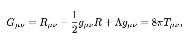
Let us go back to Eq. 5. The next step is to find the function β(r) corresponding to this metric and for that, we need Einstein’s field equations (EFE) given by:

where:

• The second-rank tensor R is called Ricci tensor and it measures by how much the geometrical properties of spacetime are different (locally) from that of the usual space (Euclidean).
• The tensor g is the metric tensor:

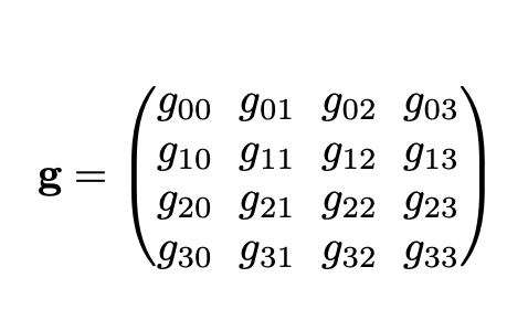
In the simplest case, that of a flat Minkowski space, the metric tensor g is:

• The scalar R is the scalar curvature R (the trace of R).
• Λ, the cosmological constant, which is equal to the vacuum energy (which is related to the dark energy) and is extensively discussed in the article below:

The Worst Theoretical Prediction in the History of PhysicsDark Energy, and One of the Most Famous Unsolved Problem in Physicsmedium.com

• The second-rank symmetric tensor T on the right-hand side is the energy-momentum tensor which has the form:

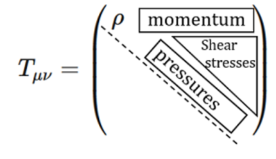
where ρ is the energy density.

Coming back to Eq. 5, we calculate the components of the tensor R and after some algebra, we obtain the following expression for dσ²:

The parameter k determines the curvature of the spatial surfaces and are commonly normalized to:

To understand the correspondence between the values of k and the geometry of the spatial surfaces see Carroll. The full metric of maximally-symmetric hypersurfaces which increase with time is called the Robertson-Walker metric

To find a(t) we need to apply the EFE. Let us follow Carroll and make the following choices that leave the line element unchanged:

Note that:

• a(t) is dimensionless
• r has the dimension of distance
• κ is not restricted to +1, 0, -1

The RW line element becomes:

Now, we can use the EFE to derive the differential equations for the scale factor a(t). Let us first write down the right-hand side (RHS). The usual choice is to model the matter and energy on the RHS of the EFE as a perfect fluid which is at rest in comoving coordinates. The tensor energy-momentum T becomes:

where ρ is the mass-energy density and p is the pressure. A perfect fluid is fully characterized by its density ρ and its isotropic pressure p both in its rest frame. It has the three following properties: it has no shear stresses, viscosity, or heat conduction (see this link).

Using energy conservation, which is given by the ν=0 component of:

we obtain:

If p/ρ is equal to some constant w the equation can be immediately integrated. We obtain:

Types of Cosmological Fluids

The most common forms of cosmological fluids are:

• Matter (including dark matter): non-colliding nonrelativistic particles with zero pressure. Examples include usual stars and galaxies. The a-dependence is just the decrease in density due to the universe expansion:

• Radiation: electromagnetic radiation and particles with mass but moving very high speeds (becoming essentially photons):

• Vacuum energy:

Note that with the simple T in Eq. 19, we can describe matter using only two quantities: its density ρ and pressure p both depending only on a(t)

Using the EFE, we obtain after some algebra the following equations for a(t).

If we make the substitutions

we obtain:

If a(t) obeys Eq. 27, Eq. 18 is called the Friedman-Robertson-Walker metric.

Density Parameter

The density parameter is a useful quantity to determine the shape of the universe. It is defined as:

The geometry of spacetime depends on the value of Ω:

• Ω<1 corresponds to the open universe
• Ω=1 corresponds to the flat universe
• Ω>1 corresponds to the closed universe

Dynamics of The Scale Factor: Solving Friedmann Equations

As shown at the beginning of the article, the energy of the universe is composed of different species which, following Carroll, I will index with the subscript i. If we know:

• the energy for each i
• the i-th equation Eq. 29 below (for all species of energy)
• the spatial curvature κ
• the cosmological constant Λ

we can exactly solve the first Friedman equation, for example, supposing all energy components evolve as power laws:

Comparing with Eq. 22 we obtain the following relation:

Following Carroll, we can treat the contribution of the curvature as a fictitious kind of energy density with w=-1/3 and n=2. This allows us to write elegantly:

where H is the so-called Hubble parameter.

Now, in the expansion of the universe different phases are dominated by different types of energy densities. Using Friedmann equations we obtain:

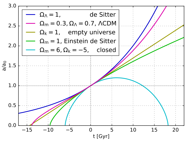
The usual analogy with the inflating balloon and an expanding Universe is shown in the figure below (the motion of galaxies corresponds to the motion of the dots).

The Big Bang

All these solutions have in common a singularity at a(t=0) = 0. This singularity is called the Big Bang. Three things must be mentioned:

• The theory of the Big Bang does not describe an explosion into a spacetime that already existed (in contrast to what many non-specialists believe).
• Stephen Hawking and Roger Penrose proved that the presence of the singularity does not occur only for FRW universes but for any universe with non-negative pressure p and positive energy density.
• At a=0 the energy density becomes infinite, and therefore general relativity is not valid at this point (one would probably need a quantum gravity theory to understand better what is happening there).

Thanks for reading and see you soon! As always, constructive criticism and feedback are always welcome!

My Linkedin, personal website www.marcotavora.me, and Github have some other interesting content about physics and other topics such as mathematics, machine learning, deep learning, finance, and much more! Check them out!