Chaos theory is potentially one of the most controversial fields in mathematics. Not because of the choice of axioms or some of the results, but due to the fact that no-one can agree what chaos actually means.

In Gleick’s book Chaos, the author interviewed a whole bunch of chaos scientists (chaosists?) and not one of them could agree on a definition of chaos.

The definition given in most pop culture media is the butterfly effect:

The flap of a butterfly’s wings in Brazil can set off a tornado in Texas

This means that given a very small change to a system, we can achieve wildly different outcomes.

Unfortunately, as with most things in mathematics, it is never quite that simple. The butterfly effect is used to demonstrate sensitive dependence on initial conditions and is one of three requirements for a system to be called chaotic under Devany’s definition of chaos — one of the most widely accepted definitions. The three components are:

1. Sensitive dependence on initial conditions
2. Topological transitivity
3. Dense periodic orbits

In this article we will explore all three of these requirements and get to the root of what chaos truly means. But first I present:

A crash course in dynamical systems

If you have already met dynamical systems, feel free to skip this section and start reading again at Sensitive Dependence on Initial Conditions.

When we talk about a system, in this context we mean a dynamical system which (for our purpose) comes in two flavours: continuous time systems and discrete time systems.

Continuous time systems are defined via an ordinary differential equation (ode)

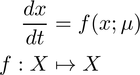
Where f is a sufficiently nice function (we usually require something like (uniformly) Lipschitz continuous) and is possibly allowed to depend on some parameter mu.

The space f maps from and to is called the phase space. For simplicity, we will assume the phase space can be equipped with a metric d (i.e. a way of measuring distances between points), this can then induce a topology (more generally, it is sufficient to require X to be a manifold that is locally diffeomorphic to a Banach space but that is far beyond the scope of this article). In most cases, our phase space will be a subset of Euclidean space and equipped with the induced Euclidean metric.

Given some value x₀ in our phase space, we can consider the flow of that point at a time t denoted 𝜙ₜ(x₀). If we give the ode an initial condition for x to start at then we obtain the initial value problem:

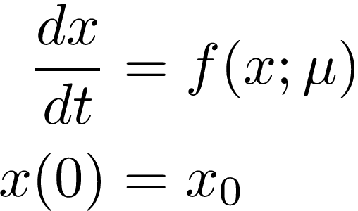
This has solution x(t), then we define the flow to be 𝜙ₜ(x₀) = x(t). We will not bother with details of conditions for the flow to exist, I will simply state that if the system is in this article then the flow will exist. (The interested reader can read about Picard’s Theorem of existence and uniqueness which states that if f is Lipschitz then locally there is a unique flow.)

We will need the definition of periodic orbit later on so might as well define it here. The orbit of a point x is the set {𝜙ₜ(x), for all time t} and so a periodic orbit is when that orbit is periodic. That is to say, for some value of t, the flow will come back to the starting condition in a loop fashion and will repeat this loop forever. You can think of, for example, the Earth orbiting around the Sun. Ignoring pesky details, the earth will loop back around and go through the point it started at.

A similar discussion can be had vis-a-vis discrete time systems. In this case we consider the governing equation

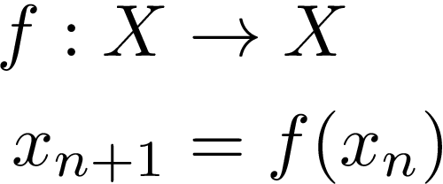
The flow of x₀ at iterate n is simply fⁿ(x₀) (i.e. f applied to x₀ n times) and it is a periodic orbit if for some n, fⁿ(x₀) = x₀.

This has been an abusively short introduction to dynamical systems with (hopefully) just the bare-bones to understand this story.

Now on to the fun stuff.

Sensitive dependence on initial conditions (SDIC)

This is probably the most intuitive of the three conditions and makes the most sense when trying to relate to chaos. SDIC was also the first part of chaos theory to be discovered.

In the 1950s and 60s, the commercialisation of computers allowed for larger and heavier computations. One field that benefited was numerical weather prediction. Edward Lorenz was heavily involved in that area and was equipped with a Royal McBee LGP-30 which he used to simulate weather patterns via a complicated set of ODEs. The resulting sequence was printed out line by line as a row of twelve numbers.

So that he could see sequences of results again, he would write down the row of numbers that occurred before the interesting part, and then the next time, he would start it off with those initial conditions from mid way through.

Though something bizarre would happen: He wouldn’t see the same sequence again. The readout would start off the same and then all of a sudden would no longer resemble the intended sequence.

What was actually happening was that the computer had an internal 6 digit precision but the printout was only to 3 digits. This rounding error meant that the starting conditions were slightly different but these differences created large long-term changes in the behaviour of the system.

What he had discovered was SDIC and the birth of chaos theory.

Very formally, the definition of SDIC is that there exists a positive delta such that for all x in the phase space and neighbourhood N of x, we can find a y in N and a time T such that:

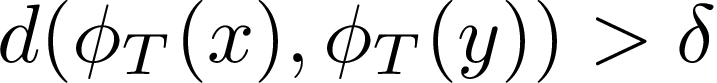
This equation holds whether we talk about discrete or continuous systems.

Less formally, this means that if you give me an initial starting condition, I can find a starting point arbitrarily close to yours whose trajectory differs by some amount.

This is sometimes referred to in literature as weak sensitive dependence on initial conditions since it just says that the flows must differ at some point. There is a stronger notion that requires the flows to at some point diverge exponentially fast.

This definition isn’t quite enough. Take for example the iterated doubling map:

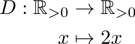
Here the n-th term is n iterates of D applied to the initial condition. It is easy to see that simply for an initial condition x₀, the n-th term is xₙ = 2ⁿx₀. Therefore given any two initial conditions x₀ and y₀, the resulting trajectory will diverge exponentially.

So whilst the doubling map is (strongly) sensitive to initial conditions, it does not behave very chaotically on the positive real line. We need some stronger conditions!

For a nice example of SDIC, look no further than a double pendulum. I am not going to prove rigorously that it exhibits SDIC because I want this story to have a sensible length also I remember going through the proof once and decided never again.

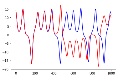
Instead I will show you this fabulous animation courtesy of Dirk Brockmann.

As you can see, the two bobs (yes that is the technical term for the mass on the end of a pendulum) start at nearly exactly the same place but after a small amount of time behave completely differently.

Topological transitivity

We have established that simply being sensitive to initial conditions is not sufficient to be chaotic. We need some stronger conditions.

We want to encapsulate the idea that the motion is ‘all over the place’. It would be sensible to require that a point cannot stay local to its starting place and that it gets flung out to explore the whole phase space.

This is where the concept of topological transitivity comes into play. It states that given an open set, it will eventually intersect all other open sets. Written in notation, this reads:

Now whilst I haven’t defined what I mean by the flow of a set, I’m sure you can understand by using the definition of the flow for a point.

Again, the definition does not make reference to whether it is the flow of a continuous or discrete map so can be applied to both.

What this means is that given a region of our phase space and enough time, it will pass through any other region. Equivalently, the orbit of U is dense in X.

A very visual example of a topological transitivity is the Baker’s transformation. It is inspired by the process of a baker kneading their dough.

We consider an iteration to be stretching the unit square and then cutting it in half and placing one half on top of the other like so:

If you stare at this for long enough, you can convince yourself that every set should eventually be spread everywhere and therefore exhibits topological transitivity.

Dense periodic orbits

Arguably this is the easiest to understand. If there is a periodic orbit, then it is dense in the phase space.

Dense means that given any point in the phase space, there is a periodic point (a point in a periodic orbit) arbitrarily close to it.

In a round about way, this ensures that there is a lot of aperiodic behaviour. Since in any subset of X, there is a dense set of unstable periodic points (instability is guaranteed by SDIC and topological transitivity) which gives rise to an abundance of aperiodic behaviour which is what we expect from a chaotic system.

NB 1: Aperiodic simply means not periodic.

NB 2: Many people disagree with this requirement. I will discuss this in the next section.

Discussion

The definition of a chaotic system given here is one due to R. L. Devaney, it is one of the most widely and commonly accepted.

It has been shown (Banks et al., 1992) that in the discrete time case, provided the phase space is a non-finite metric space then in fact being topologically transitive and density of periodic orbits implies SDIC. In an even more extreme case Michel Vellekoop and Raoul Berglund proved that if we restrict even further to (possibly infinite) intervals, then being topologically transitive implies the rest (Vellekoop and Berglund, 1994).

As I alluded to at the start of the section, there are many definitions of chaos. Peter Smith suggested that Devaney’s definition is a consequence of chaos and not a true definition itself. To name drop a few different definitions for you:

• A discrete map is chaotic if it exhibits topological entropy
• A discrete map is chaotic if it has a positive global Lyaponov exponent
• A discrete map is chaotic if at some point it maps the unit interval into a horseshoe

You might note that all these definitions talk about discrete maps, this is because you can always construct a discrete map from a continuous map using something called a Poincaré section (shown adjacent). A Poincaré section allows you to reduce the dimensionality of your system and make it discrete.

If the continuous system is chaotic then the dynamics on the Poincaré section will be chaotic.

So now you know! I think one of the most fascinating parts to this story is that unlike in a lot of mathematics, there is no obviously correct or sensible definition — it is purely a best guess at describing a physical phenomena. The direct consequence is that there are lots of conflicting notions of what chaos actually is.

To learn more about this topic, you can watch these two videos by the Youtuber Veritasium: Logistic Equation and Butterfly Effect.

I would also strongly recommend the book Chaos by James Gleick.

References

• Banks, John & Brooks, J. & Cairns, Grant & Davis, G. & Stacey, Peter. (1992). On Devaney’s Definition of Chaos. Amer. Math. Monthly. 99. 332-. 10.2307/2324899.
• Cavers, J.G. (2017). Chaos and Time Series Analysis: Optimization of the Poincaré Section and distinguishing between deterministic and stochastic time series.
• Vellekoop, Michel & Berglund, Raoul (1994) On Intervals, Transitivity = Chaos, The American Mathematical Monthly, 101:4, 353–355, DOI: 10.1080/00029890.1994.11996955