A Finite Solution to Lorentz Factor at the Speed of Light

In theoretical physics, the Lorentz factor is a term by which relativistic mass, time, and length changes for an object in motion. It is named after the 1902 Nobel Laureate Dutch physicist Hendrik Antoon Lorentz, who together with Pieter Zeeman discovered and theoretically explained the Zeeman effect. Lorentz also derived the transformation equations that would end-up playing an important role in Albert Einstein’s theory of special relativity (in 1905). This article concerns the latter of his achievements.

Lorentz factor, also referred to as the Gamma factor, is mathematically defined as follows:

Problem definition

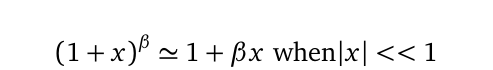
The presence of Lorentz factor in special relativity presents a monumental difficulty when estimating relativistic mass, energy, momentum, and time dilation, as the speeds tend towards that of light in a vacuum. In particular, mathematical singularities become inevitable as the square speed ratio v²/c² tend towards unity (1). It also becomes a challenge when the object(s) under study has a velocity, v that is too low compared to that of light in a vacuum. As a result, physicists have always gotten around it by taking binomial approximation of the following form:

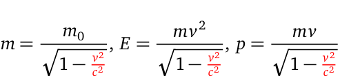
It can be seen from Eq. (1) that calculations at the constant speed (of light in a vacuum), c results in infinities. This makes relativistic and quantum mechanical operations (pertaining Lorentz factor), such as length contraction, mass, energy, momentum, and time dilation highly problematic. This was also one of Paul Dirac’s tenets when he formulated relativistic quantum mechanics. The most obvious cases to consider however, are the relativistic mass-energy-momentum equations, underpinning special relativity as formulated by Albert Einstein, which are stated as follows:

The impending question is, what exactly happens when v =c in Eq. (3)? perhaps it makes more sense if we start with the lower boundary, v = 0. The object is not in motion, and thus relativistic mass just equals the rest mass, both kinetic energy and momentum are equal to zero. However, as the object gains motion, all the three quantities gets distributed over position and time, from rest to the classical limit, before the quantum properties kicks in. In the next sections we will try to find a finite solution for the system.

Seeking a finite solution

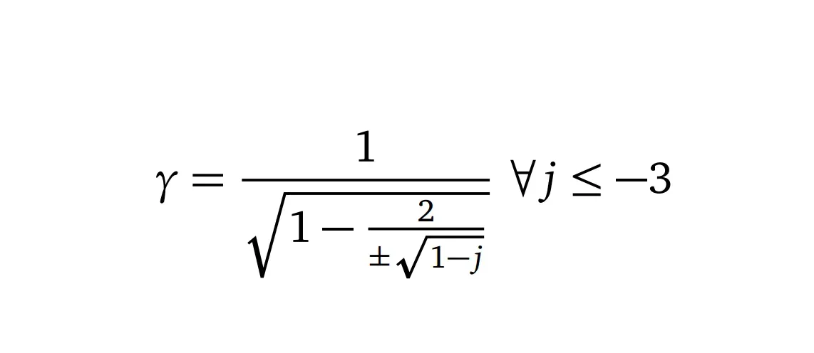
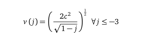
Instead of binomial approximation, what if we introduced a renormalization parameter — call this j. Renormalization is a technique used in quantum field theories to treat infinities that emerge from calculated quantities that would otherwise lead to nonsensical (infinite) results. We therefore formulate the square speed ratio as a function of this j such that:

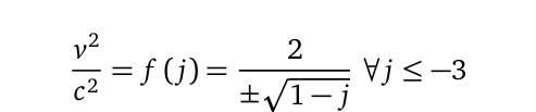
We will expound more on what j is, but for now it is just enough to know that a jvalue of -3, yields v²/c² = 1, and that is the maximum value. The theorem in Eq. (4) is also true for all values in that range, and makes sense for as long as we keep in mind theoretical limit, c that is the speed light in a vacuum. A quick test can be performed at -8, -15, -24, -35, …… and so forth.

The physical implication of renormalization

Assuming the mathematical case for Eq. (4) is settled, what do we presume to be the physical implication of the renormalization parameter j? Well, it turns out to be regime specific — meaning, it depends on the region in which the particle is located and the speed. For instance, we could define j for electrons in an hydrogen atom as follows:

Where: n is the electron shell number, or energy level, also referred to as the principal quantum number. The parameter α≃ 1/137.06 is called the fine structure constant, a dimensionless number that makes frequent appearances when dealing with elementary particles. This hypothesis can be tested with n = 1, for the ground-state electron of an hydrogen atom, and you would expect to find a corresponding value of j, and most importantly, an exact speed of the electron in that shell at about v = 2187308.1716 m/s.

The renormalization parameter can also be expressed as a function of speed itself, meaning that for any (non-stationary) object whatsoever:

To test the validity of Eq.(6), you would also want to plug in any known value of the speed, v, and estimate j, which may then used to calculate the energy level of an electron in hydrogen atom. From the earlier explained example, when v = c, jmust necessarily reduce to a maximum value of -3.

Comparison with Dirac Equation

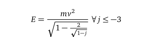
In order to successfully apply the derived renormalization, it is noteworthy that the denominator of Eq. (4) takes both negative and positive values. Meaning that, we take the former in all the cases such that the speed is always returned by the following function:

Replacing Eq. (7) back in any of the mass-energy-momentum terms in Eq. (3) effectively eliminates the singularities. With the energy equation for instance, it results in the following form:

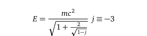
The theoretical implication here is that at the speed of light in a vacuum, the particle’s energy must reduce to the following form:

Meanwhile, Dirac’s exact energy equation predicts relativistic quantum mechanical properties of hydrogen atom using the following method:

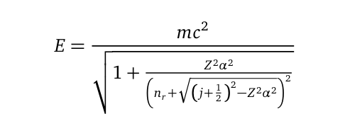
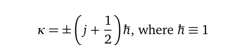
Where Z²α² is a small non-integer number, while the principle quantum numbers in Dirac equation Eq. (10) are described by the linear relation n=nᵣ + κ. Where nᵣ is the quantum number at a specified radius, r, and κ is a non-zero integer that is in turn given by the relation:

NB: The notation j in Eq. (9-10) is different from the one described in Eq.(4–9). It is thus strictly specific to Dirac’s formulation.

Notice the similarity between Eq. (9) and (10), especially the second term under the square root in the denominator of the RHS. Based on this observation, we can therefore make the following conclusions:

Conclusion

We have derived a simplified finite solution to Lorentz factor. The key takeaway here is that the square speed ratio that usually presents a challenge when dealing with Lorentz transformation equations, has a finite solution that can be leveraged and used to perform relativistic quantum mechanical calculations such as: time dilation, length contraction, mass, energy, and estimation of particles momenta. However wound up Dirac’s equation is, it still provides an exact method for hydrogen atom. It is therefore noteworthy that this is not a complete replacement of Dirac’s equation, but a complementary one since it does not predict other estimates such as the quantum “spin” effect even though it predicts the speed accurately.