This article flows out of a video conversation between the YouTubers and mathematicians Grant Sanderson and Matt Parker (references below) and an email conversation between myself and a friend of mine: Peter Gaffney as we explored our own solutions to this beguiling puzzle.

Exploring different approaches to this seemingly impossible problem reveals some interesting connections between various branches of mathematics including logic, set theory, multidimensional vector spaces and even category theory.

Outline of the Puzzle

You and a fellow prisoner are imprisoned in a dungeon and are facing execution. As is usual in these problems, the prison warden has both a love of recreational mathematics and an unusual amount of judicial latitude when it comes to deciding your fate. They want to give you and your cellmate a chance of freedom but don’t want to make it too easy for you.

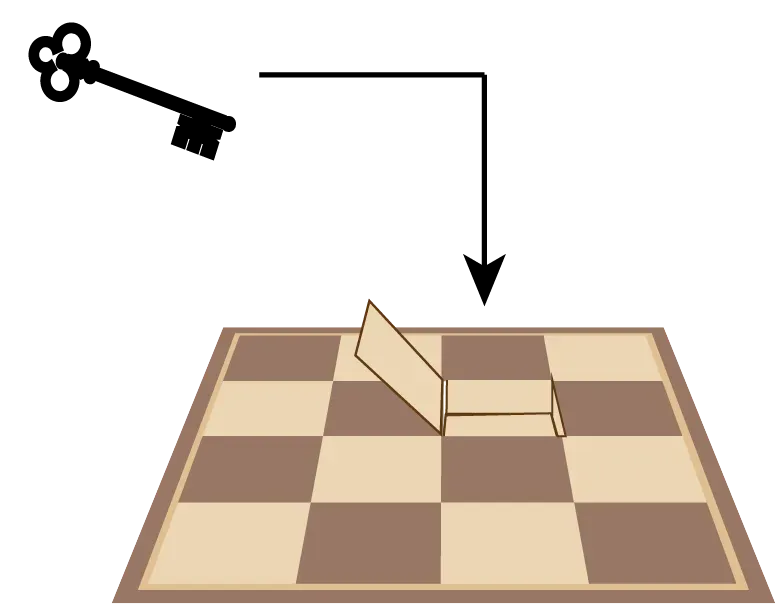
They have a chessboard where each square is covered by a coin — either heads or tails. Moreover it’s a special chess board with a hidden compartment in each square. A single one of these squares contains a symbolic key to the jail and freedom for you and your cell companion. You will know which square contains the key and your fellow prisoner has to guess.

The rules are as follows:

(1) You and your cellmate can discuss how to encode a message using the chessboard but the prison warden can hear and understand everything that you say.

(2) Once you have decided on a system, your companion leaves the room.

(3) You observe the prison warden hiding the key in one square and then arranging the 64 coins as heads or tails however they deem fit — presumably trying to frustrate your system.

(4) You then turn over exactly one coin on the chess board and leave the room.

(5) Your companion re-enters the room, without having any opportunity to see or communicate with you. He observes the chessboard and the arrangement of coins and points to the square where he believes the key and freedom reside.

(6) Nothing sneaky is allowed on pain of immediate death i.e. This is a pure logic problem- there is no meta game. Paper and Pencil, calculator and plenty of time are available to you and your cellmate if necessary.

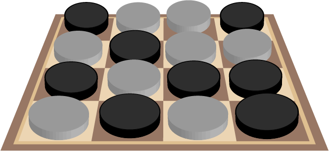
In order to make our diagrams easier to understand, we’ll use dark and light counters to represent heads and tails and limit ourselves to a 4 x 4 chessboard with 2⁴=16 squares. However everything we discover will apply equally well to a standard chess board with 2⁶=64 squares or even far larger chessboards provided the total number of squares is a power of two.

Some Properties of the Problem

The prisoner warden gets to set all the coins on the board and we only get to flip one to convey our message- a tiny signal in all that noise. At first glance this seems completely impossible but let’s start by understanding what is relevant in our puzzle and what we can discard. Then we’ll see if we can start with a simpler version of the problem.

For starters, the geometry of the chessboard is irrelevant, because we are not dealing with chess moves or anything else that would make the relationship of squares to each other important. The squares could all be in a row, in a four dimensional 2x2x2x2 hypercube or any other configuration. Additionally the order of squares doesn't matter as long as we keep track.

In some sense, the chessboard must encode the 4 bits of information required to specify the row and column of the key square. Given that the prison warden will have chosen a configuration either at random or maliciously, some or all the bits encoded may be wrong. So it must be possible to choose a coin to flip (represented here by the counter changing color) that will fix the wrong bits without impacting the correct ones. In the case where the chessboard already encodes 4 correct bits, there must be at least one square that has no effect on the 4 bits when its coin is flipped.

A single square chess board (1 = 2⁰) has no information to transfer because the key can only be in that square. The first non trivial case is two squares (2 = 2¹). We will start with this and generalize using 4 distinct approaches to get to a solution.

Fell free to take a pause before continuing. It’s a fun problem that is very rewarding to mull over.

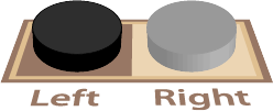
Let’s start by solving the two square case which, based on the hints above, is relatively simple. We need one square that does nothing when we flip its coin (aka change its counter )- let’s choose the one on the left. This means that the right square needs to encode the location of the key. Let’s choose light for left and dark for right. When the warden has finished with the board, if the right-hand coin indicates the incorrect square for the key, we flip it. However if it is already correct, we flip the left-hand coin which has no effect on our key location message.

Now we’re ready to scale up to bigger boards and consider various approaches. These approaches can be read separately if you want to dip in and out of this article.

Approach A: Hypercube

Let’s imagine our squares to be arranged into a 2x2x2x2 tesseract — a 4 dimensional hypercube of side length 2.

If we consider each dimension separately, we will have 4 separate pairs of squares and we already know how to solve a single pair of squares. However we do have an issue as we no longer have single coins for each square. Each square has behind it a collection of 2³=8 coins, one for every possible combination of the other dimensions. Somehow we need to be able to aggregate all these to produce a single virtual “coin” on the right representing that dimension. A single coin is an odd number which suggests the possibility that we regard the virtual “coin” as dark if there is an odd number of dark coins in this collection of 8 and light otherwise- this is often called parity. To make this clearer, let’s temporarily drop to 2 dimensions and show the parity coins that are aggregated from a collection of two coins in this case, as shown in Diagram 4.

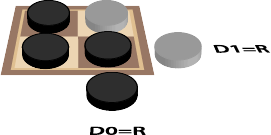
We can change from odd to even for our dimension or visa versa by flipping either of the 2 coins. Even nicer, the dimensions are of course independent. There is a coin for every single combination of dimension coordinates. So we can work out the coordinate of the coin to flip (left or right) separately for each dimension. If the current parity coin for a dimension Dₓ does not indicate the location of the key in that dimension, we can change the parity by flipping a coin that is on the right for that dimension: Dₓ=R. If the parity already indicates the location of the key in that dimension, then we flip a coin on the left: Dₓ=L. When we have done this for all available dimensions, we will have unique coordinates for the coin to flip.

So we have a way to solve a 2x2 square or indeed our 2x2x2x2 hypercube. But how to we map the chessboard squares onto this hypercube? One approach is to drop down to a single dimension first, as in Diagram 5.

We can then use the algorithm that many programming languages use for implementing a multi-dimensional array in a linear address space. This involves a form of recursive nesting which should be fairly obvious from Diagram 6.

Putting all this together, we get the labeling shown in Diagram 7.

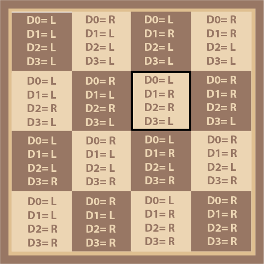
Now we can produce the virtual coins for each dimension Dₓ by working out the parity of each collection of 8 coins where Dₓ=R as shown in Diagram 8.

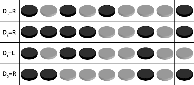
The board currently codes for the position: D₀=R, D₁=L, D₂=R, D₃=R. We want it to code for the position: D₀=L, D₁=R, D₂=R, D₃=L. D₀, D₁ and D₃ are incorrect. We indicate a change with R and can leave the parity of a dimension alone with L so we can fix the position encoded by the board by flipping the coin at D₀=R, D₁=R, D₂=L, D₃=R.

Approach B: Binary

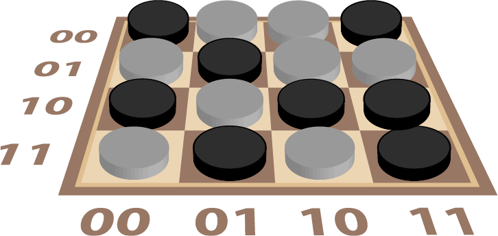
Let’s consider our board again but label our rows and columns. Instead of using the usual letters and decimal numbers, we label both with a pair of binary digits (bits) in Diagram 9. This highlights that we need to somehow encode the position of our key (in the third column of the second row) as 0110.

With our two square chessboard, we can label the first square 0 and the second square 1 but how do we extend this to larger chessboards? We can number pairs of squares 0 and 1 and then do the same for pairs of pairs and so on as in Diagram 10.

And yes, we’ve just reinvented binary counting meaning that each of the squares on our chessboard can be labelled by a 4 digit binary number as in Diagram 11.

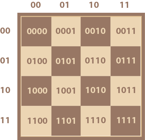
Because the width of the chessboard is an even binary number: 4=2², this gives us a simple pattern when we consider the squares that have one in various positions. If we use Blue for bit 0 or D₀, Red is bit 1 or D₁, Green is bit 2 or D₂ and Yellow is bit 3 or D₃ we can more easily see how the chessboard is divided into bands as shown in Diagram 12.

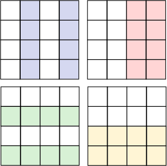
In a sense this is the result of collapsing our 4D tesseract into 2D. Two of the dimensions represented by the pink and yellow bands have maintained their left right symmetry. The other two dimensions have had their symmetry broken by folding. We assigned binary numbers to each square on the chessboard but another way of looking at these numbers is as bit vectors: that is the coordinates of a coin location in a 4 dimensional vector space as in Equation 1.

As with all vector spaces, a general vector here is a linear combination of the independent basis vectors. However the scaling factors are all either 0 or 1 which implies that each basis vector is part of the linear combination or it is not. In effect, this vector space describes the 2x2x2x2 tesseract from Approach A.

Now we could just calculate the parity of each band in Diagram 12 as before i.e. we could check if there is an odd or an even number of dark coins in each band. However we don’t actually need to count, we can just toggle between odd and even every time we encounter a dark coin in the band — this is effectively modulo 2 addition or can also be considered as a NOT operation where 0 and 1 represent False and True. We only want this NOT operation to take place when we encounter a dark coin that is in a band represented by a 1 bit in the appropriate position. There is a neat way to do this using an Exclusive OR operation.

One way of looking at exclusive OR is as a controlled NOT with a control argument and a data argument. When the control argument is zero, nothing happens to the data argument. However when the control argument is one, the data argument gets inverted either from 0 to 1 or 1 to 0. Finally the exclusive OR operator available in many computer languages doesn’t just operate on a single bit. It can operate on two bit vectors where the corresponding individual bits in each vector are exclusive ORed to get the result.

So all we need to do is the following. Scan the board from top to bottom calculating a cumulative value which starts as the vector 0000. Each time we encounter a dark coin, we perform an exclusive OR of our square’s location label with the current cumulative value to get the new cumulative value. At the end, this cumulative value represents the location of a square. If we use the board in Diagram 9, this turns out to be 1011. However we need the board to represent the third column of the second row or 0110. To list the bits that need to be corrected, we simply exclusive OR these two vectors together to get 1101 which is the location of the coin that we need to flip.

You may wonder whether there are other logical operations we could choose when assembling the cumulative value that will indicate the key location. In practice, the choice of operator is quite constrained. We want each bit location to be independent which rules out operations involving borrows or carries. Operations like AND or OR aren’t fit for purpose either, because AND and OR ignore their second argument when the first one is 0 or 1 respectively. This makes it possible for a malicious warden to choose coins that will lock out information from a region of the board where he can then hide the key. So we need a logical operation that is always sensitive to changes in each input argument. That only leaves Exclusive OR which returns True when its arguments are different or its inverse: Equivalence which returns True when its arguments are the same.

Approach C: Exceptions to the exceptions

To ease into this approach, keep in mind the rule for leap years which has a basic condition modified by subsequent conditions:

It’s a leap year if the year is divisible by 4 unless (the year is divisible by 100 unless (the year is divisible by 400)).

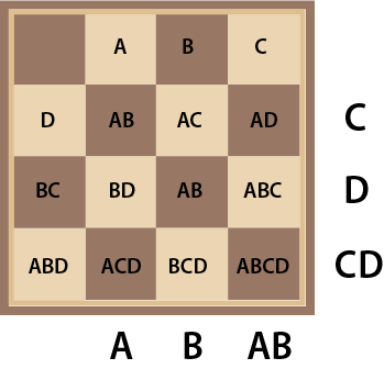
On the chessboard in Diagram 13, we use combinations of letters to label the rows and columns. For example A by itself represents the 2nd column; B by itself represents the the third column; A and B together represent the 4th columns and no A or B indicates the first column. This means that A can indicate either the second or the forth column. The squares are also labeled with combinations of letters. By analogy with the leap year rule we have the following (involving all the squares that contain A in their label):

A square is set if it has a black “coin”. We are referring to an A column if square A is set unless AB is set unless AC is set unless ABC is set unless AD is set unless ABD is set unless ACD is set unless ABCD is set.

The rules for B columns and C and D rows are very similar. English is a little vague when it comes to logic but X unless Y could be regarded as X and not Y. So if X and Y are invited to a party but really don’t like each other we might have the rule X unless Y and Y unless X, more formally (X and not Y) and (Y and not X) which is exclusive OR. Because our Xs and Ys are disjoint, the full rule of X will give us one half of the exclusive OR and the full rule for Y will give us the other half.

When my friend Peter came up with this approach, knowing my love of Pascal’s triangle, he was keen to point out the numbers of squares are 1 with no letters, 4with one letter, 6 with 2 letters, 4 with 3 letters and 1 with 4 letters which is a row of the triangle: 1 4 6 4 1.

To understand why this is, let’s look at the simpler 2x2 example in Diagram 14 . We are just interested in numbers of letters, so we can replace our As and Bs with the more general X and we get a graphical representation of (1+x)² and another row of the triangle: 1 + 2 x+1 x²

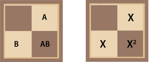
By analogy our 4x4 would represent (1+x)⁴ but that does suggest we should reorder our square labeling as in Diagram 15. Please note that this might look more elegant, but the order of the squares is irrelevant and their labeling doesn’t need to match up with the row and column labeling used to identify the key location.

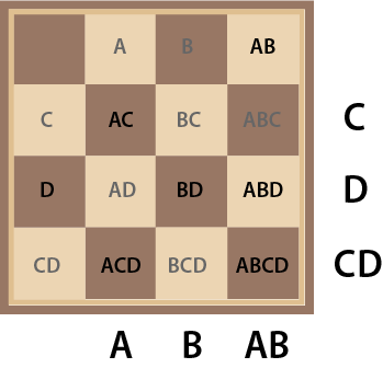
When we evaluate the four rules for the board configuration shown in Diagram 9, we discover that the rule for B produces False while the rules for A,C and D all produce True indicating the second column of the forth row. The key is located in BC so we need to changes the results of rules AB and D which we can do by flipping the coin at ABD to light color.

We can emphasize how the rows and columns overlap by using colors: blue for A, red for B, green for C and yellow for D as in Diagram 16.

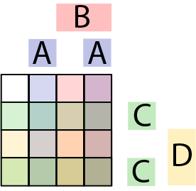
While both A and C are in two pieces each, this is basically a Venn Diagram for 4 sets similar to that in Diagram 17.

Diagram 16 keeps all the overlaps in the Venn Diagram the same size. In two dimensions, this is only possible with some non contiguous sets in the diagram. Of course Approach A is also effectively a Venn Diagram in 4 dimensions where all the overlaps are the same size.

Nothing to do with our problem here, but interestingly, when the consistency of overlap size is relaxed, it’s possible to get some remarkably symmetrical Venn diagrams in 2D such as this gorgeous 11 set example:

Back to our chessboard where we can go even further. Let’s say A,B,C and D represent single element sets so that A={0}, B={1}, C={2}, D={3}, then all the squares on the chessboard reading from top left to bottom right represent the entire Power Set for the set {0,1,2,3} as shown in Equation 2. A Power Set is the set of all possible subsets of a given set.

Thus one can see how a power set for a set with n elements itself has 2ⁿ elements. As each of the subsets represents one way of choosing k elements from a set with n elements, we have another reason for Pascal’s triangle in Equation 3.

Our chessboard, by having some dark coins, has selected one particular subset from the Power Set. This subset is itself a collection of elements which themselves are subsets of {0,1,2,3}. The subset selected by the chessboard is in fact (A∪B)⊕(A∪C)⊕D⊕(B∪C)⊕(A∪B∪D)⊕(A∪C∪D)⊕(A∪B∪C∪D). In order to reduce this expression, we’re going to make use of the identities in Equation 4.

The first two rules in Equation 4 work in tandem to ensure that an odd number of Xs exclusive ORed together produces an X whereas an even number produces the null set. The third rule distributes exclusive OR across union (also called disjunction). It’s worth emphasizing that this is not a general rule and only works because Y and Z are disjoint. Not relevant here but there is a general distribution rule involving exclusive OR shown in Equation 5:

Intersection (also called conjunction) distributes over exclusive OR. In fact these two operations form the field GF(2) where intersection is equivalent to modulo 2 multiplication and exclusive OR is equivalent to modulo 2 addition.

So now, with the help of our identities, we can do the reduction as shown in equation 6 which indicates the square ACD as expected.

So to sum up, the chessboard is the set of all possible subsets of the set of 4 elements- the power set of {0,1,2,3}. For a set of n elements, the power set contains 2ⁿ elements and so there are 2⁴=16 squares on the chessboard , one for each subset. Moreover the dark coins select a set of these subsets which is in fact a subset of the power set- one of 2^(2^n) = 2¹⁶ = 65536 such subsets. Our algorithm for identifying the key square from a board configuration is in fact a mapping from a subset of the power set of {0,1,2,3} to a subset of {0,1,2,3}.

If you’ve ever played Reversi or Othello, you’ve engaged in a power struggle over a power set where one player is striving to fill the set and the other to empty it. :-)

In approach B, each square was identified by a unique binary number which could also be regarded as a bit vector. In approach C, each square is identified by a unique set. This is not that surprising because in programming languages, bit vectors are often used to encode sets that may only contain small numbers. The typical word length in a modern computer is 64 which allows us to efficiently encode sets that contain as elements any of the numbers from 0 to 63. For sparse sets with lots of missing elements, a hash table is more efficient because a 0 bit is not needed to record each absence.

Approach D: Self Composition

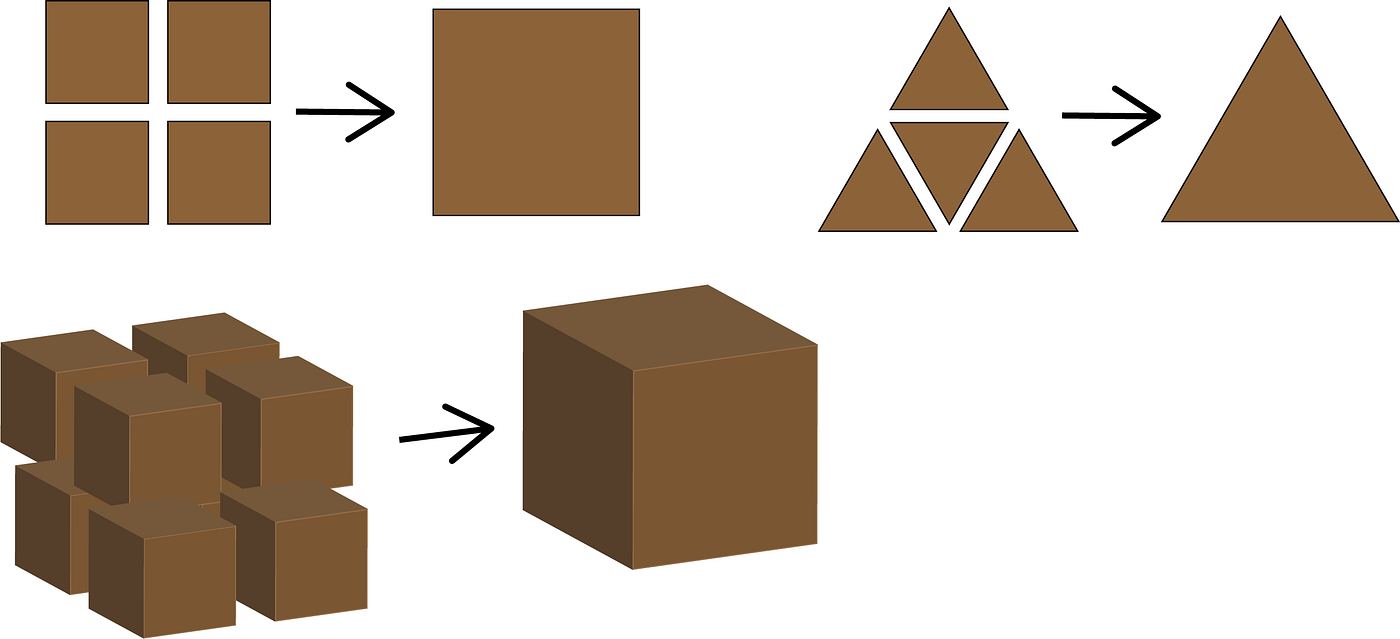
When Category Theory was developed to formalize fundamental structures in various branches of mathematics, it was so abstract that few thought it would ever have a practical application. Yet very quickly the idea of Composition, for example, has turned out to be an extremely powerful way of addressing problem domains using Functional Programming. You can get a very informal idea of self composition from Diagram 19. Here we see that a square can be composed from 4 smaller squares and a triangle can be composed from 4 smaller triangles, 3 at the corners and one upside down in the middle. Hexagons can tile the plane but they can’t self compose. Extending to three dimensions, we can see that a cube is composed of 8 smaller cubes. It might seem that a tetrahedron could be composed from 5 smaller tetrahedrons, one at each corner and one upside down again in the middle but that shape in the middle turns out to be an octahedron.

But I digress. How can self composition help us with our chessboard? Let’s look at the simplest non trivial case of two squares again as in Diagram 3. Is there some sense in which this two square chessboard can be composed from two additional two square chessboards? We can obviously discard features not relevant to our problem like the size and color of the squares. In fact we can discard everything but the coin on the right which tells us which square the key is under (dark=right, light= left). In the case of a two square chessboard containing a two square chessboard in each of the left and right squares, things work nicely because each two square chessboard simplifies to a coin. But how do we generalize this to multiple levels? The answer is to consider a single coin as a special case of a stack of coins.

Rather than nesting all these chessboards in our diagrams, it will be a lot neater to show the whole lot as a binary tree. Here each step of composition occurs moving up as we combine two squares containing two stacks of coins to form a single stack of coins as in Diagram 20 which will make more sense shortly.

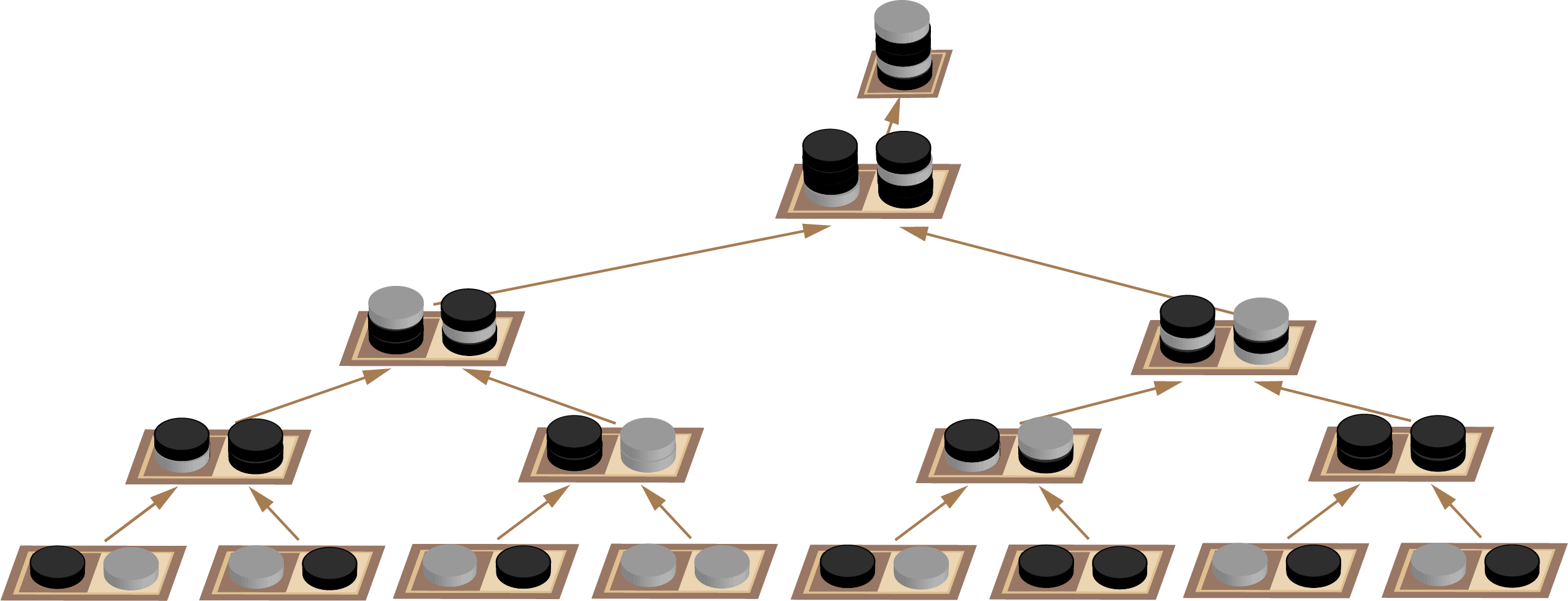
Finally we get to the crux of this approach: we need a rule for combining the stacks of coins. We know the rule at the lowest level already. Make a stack of one from the coin on the right.

We’re going to need 4 coins when we get to the root which we can then use to work our way back down the tree using light for left and dark for right. I got stuck initially with this method until I realized that an extra coin was needed at the top of the stack as a form of eager evaluation. Our top coin is the parity of the entire board at that node in the tree. Ordinarily this is of no interest because we can’t use it to communicate anything to our cellmate. We are obliged to flip a coin so the parity of the complete board will always change from odd to even or even to odd beyond our control. However if this is not the root node of the tree, the parity of the complete board will be of use if that board turns out to be on the right hand of the next node up. If it is on the left hand, the whole board parity is discarded. Producing intermediate results that we might need and discarding them if we don’t is a characteristic of parallel systems.

This all leads us to the rule for combining stacks down in Equation 7.

Here ⚬ represents the operation of composing two stacks of coins to form a new stack that is one higher. Stacks of coins are numbered from the top down. [0] indicates the top coin and [>0] indicates every coin except the top. The comma represents concatenation where multiple stacks are merged to form a single stack. Finally ⊕ represents exclusive OR which can be applied to two single coins. However it can also be applied to two stacks of coins where this implies that the operation is actually being applied to corresponding individual coins in each stack.

⊕ requires its arguments to have the same number of coins. The result in other cases is undefined because there will be at least one coin with no corresponding coin in the other stack. To avoid this undefined behavior, we need to always combine stacks with the same size. This implies that that the tree we are working with needs to be perfectly balanced i.e. have the same depth everywhere. This in turn means that the chessboard can only contain a number of squares that is expressible as a whole power of two. 3Blue1Brown has a very neat alternative justification for this limitation involving graphs and coloring.

The rule in Equation 7 might be easier to understand if we work through an actual example with coin stacks as down in Equation 8.

Next we need to build up a stack of coins corresponding to the location of the key as shown in Diagram 21. Each time we move up the tree we add a coin to the stack. If we entered the node from the left, this coin is light and if we entered from the right it is dark.

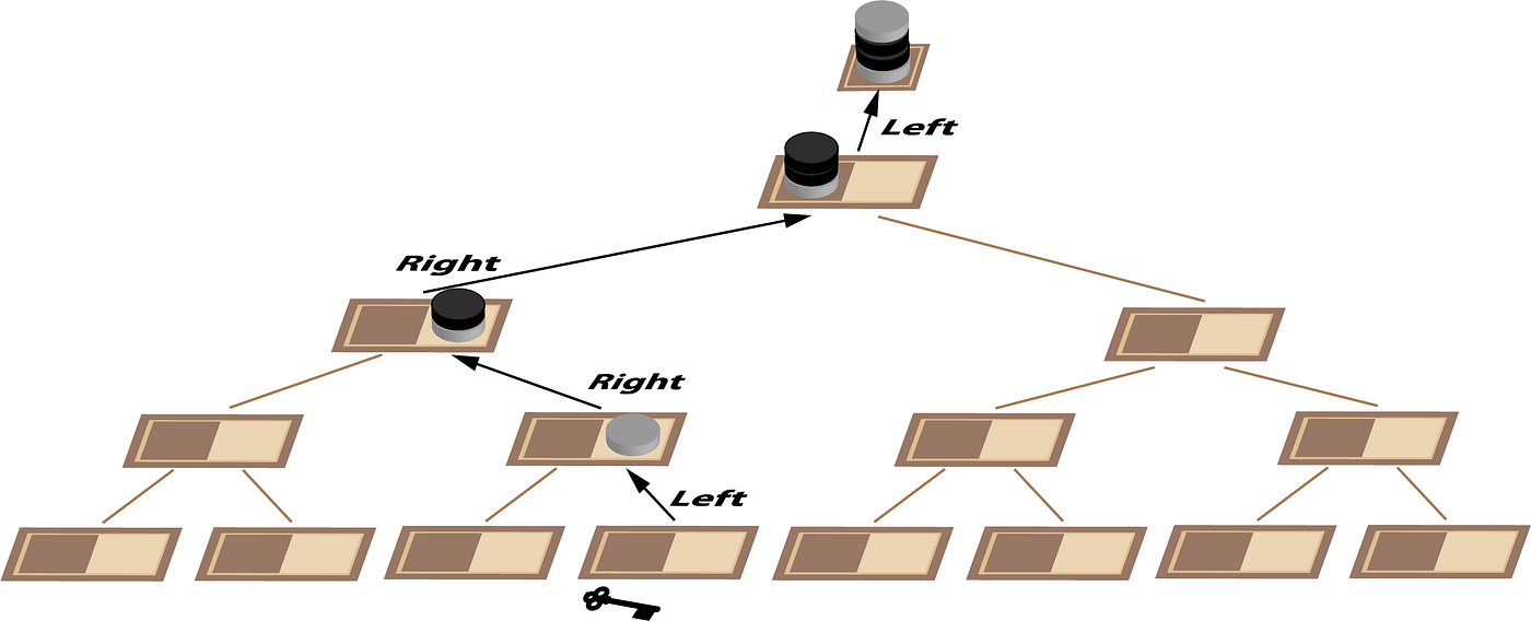
Now (Equation 9), we take the stack of coins assembled in Diagram 21, discard the top one for whole board parity and exclusive OR this stack with the stack that we generated in Diagram 20.

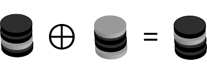
We now have the stack of coins that address the square on the chessboard containing the coin that we need to flip. We walk down the tree (Diagram 22), taking the top coin off the stack at each step and going left if it is light and right if it is dark. And that’s all there is to it. :-)

This might seem more complicated than the other approaches. However it has one useful feature- it is a parallel algorithm. For the last half century, we have been thoroughly spoiled by Moore’s law where processor speed has been doubling roughly every two years. These halcyon days are coming to an end, so we need to move away from doing things one at a time. Algorithms and their implementation will need to be inherently parallel to address the problems in our future.

If you’d like to see how to go from these binary trees to modular logic networks that can perform the individual tasks for both prisoners, do let me know in the comments.

Practical Application: Huffman Coding

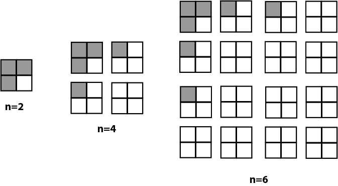
This is not just a fun problem in recreational mathematics. We can turn it on its head to implement Huffman coding — an early form of error compression used in digital communications and recording. This time the arrangement of coins on the chessboard represents a message and the symbolic key is always under square 0000 in the top left corner. A single coin can then be flipped representing an error in the message. Using our existing algorithm we can determine which coin this is and flip it back in order for the 4 bits to address square 0000 again i.e. even parity on the right for every dimension.

In order to always achieve even parity, we need a single coin for every dimension that can be flipped if necessary to make the number of coins on the right even. These parity squares are not available for data. Also the 0000 square is not available because an error can’t be detected here. For a small number of dimensions this is ridiculously inefficient. For example for 2x2 board, we have only 1 data bit. However each time we add a dimension we double the number of bits available and only have to subtract 1 for use as a parity bit. This deal gets better and better every time we double the block size so the efficiency is (2ⁿ -n -1) / 2ⁿ which works out to 69% data squares for our small chessboard (n=4) and 89% data squares for a normal sized chessboard (n=6). However if we go too far we will make the probability of double or triple errors too likely and these can’t be corrected by this scheme.

3blue1brown explores Huffman Coding in more detail here. The Exclusive OR operation is key to the efficient operation of this algorithm. This operation has all sorts of other cool applications. It can be used to encrypt a message by exclusive ORing the data with a random key of the same length. The receiver repeats the operation to recover the data. It can allow one drive to backup two other drives in some forms of RAID storage. It truly is the star of boolean algebra.

Conclusion

So having investigated these various approaches, we may have developed an intuition for the problem space. We can change which squares we use to encode different bit combinations. We can aggregate tails instead of heads; We can aggregate the coins on the left instead of the right. We can use the equivalence operation instead of exclusive OR. However all these just represent symmetries. It makes no fundamental difference to the underlying solution regardless of which of these we choose. And of course all our various approaches used different mathematics to converge on the same solution.

As far as this problem is concerned, there is no difference between a binary dimension in a vector space, a binary digit, a set or indeed a level in a perfectly balanced binary tree.

For other takes on this wonderfully evocative problem, have a look Matt Parker and Grant Sanderson’s video conversation discussing solutions in an actual dungeon (well almost). There is an interactive version of approach B available here. And if you want to delve even deeper, have a look at the topics for Information Theory, Entropy and Combinatorics in Wikipedia.