This story will give you an introduction to how to model technical systems. It covers why modeling is so important for engineers, some basic techniques, and an example of a technical system describes via an ODE.

Why modeling is so important as an engineer

Just to make this clear right away: Not every engineer is modeling technical systems at his job, by far. However, in my opinion, it is a more and more important skill to master. Due to the rise of cheap computational power, Computer-Aided Engineering (CAE) replaces or supports different parts in classical product development. And in the end, it mostly breaks down to the point where you need to build a model depicting the reality with adequate accuracy.

Essentially, all models are wrong, but some are useful (George Box)

Modeling consists basically of two aspects. On the one hand, we have the mathematical/technical part where we translate a technical system or concept into something we can solve, with the help of computational resources or by hand. On the other hand, we have a more challenging aspect of modeling. The engineer has to decide how detailed his model has to be to approximate the reality adequately. All the techniques and methods available to analyze and model systems are useless if you focus on the wrong model. Geroge Box really nailed it. No model has ever predicted something 100% exactly, there are too many unknown variables in reality.

Just to mention a few important fields of engineering with regards to modeling (technical) systems:

• stress analysis and Finite Element Analysis (FEA)
• Computational Fluid Dynamics (CFD)
• Multibody Dynamics
• Controller Design
• Climate Prediction
• Economics

Basic techniques & math¹

The goal of the modeling process is to create a mathematical formulation which describes our system. The formulation can then be used e.g. to describe how our system reacts to a unit step input over time.

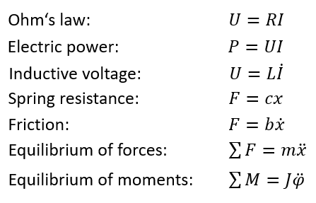
To build a model of a technical system, you use basic linear and non-linear equations of laws of physics and combine them. Figure 1 shows a few examples of commonly used equations to describe a technical system.

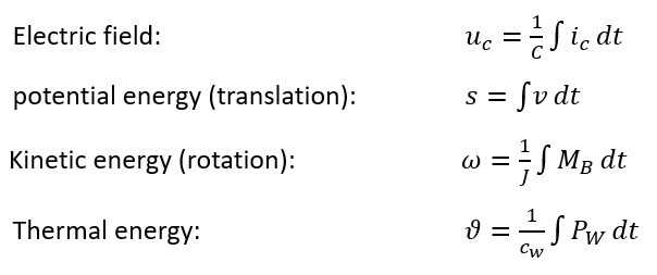
However, the core of a technical system and therefore the model are the equations that describe the energy inside the system. E.g. in classical mechanics, this is the kinetic energy of the system, in electronics this could be a capacitor, and in thermodynamics simply an equation describing the heat of a system. Figure 2 shows the most common equations used to model the energy of a system. These equations e.g. are used to set up the block diagram.

If we now have analyzed our system and have written down all of our equations needed, we have two options to continue with modeling.

1. Set up the Differential Equation
2. Set up the block diagram (and the transfer function)

Both methods will lead to a proper solution. I will focus on the first method here. The second one is necessary to model and solve systems with simulation software like MATLAB/Simulink. The differential equation can still be solved numerically if the analytical approach is not looking promising (what is mostly the case…).

Furthermore, I think understanding the basic concept of modeling a system via a Differential Equation definitely helps to get a deeper understanding of systems. So let’s have a look at an example where everything is put together!

A common example

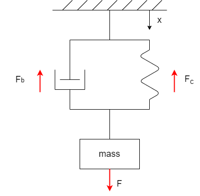
One of the most common examples in system theory is a mechanical PT2-System modeled via a mass connected to a spring and a damper. Figure 3 shows the technical sketch of the system. The input is an external force F and the output (that’s what we want to describe) is the displacement x.

In order to model the system we need an equation that describes:

1. The equilibrium of forces
2. The damper
3. The spring

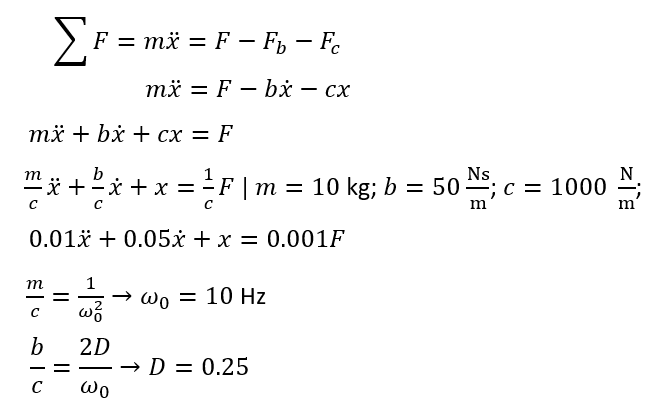
The equilibrium of forces is our bases where we input all the equations necessary to describe the output x. Figure 4 shows how the ODE is set up. If we put in some values for our three parameters mass, damping rate, and spring rate we get a final ODE describing our system. If we normalize the ODE so that x has a factor of 1 we can calculate the natural frequency and Lehr’s damping measure.

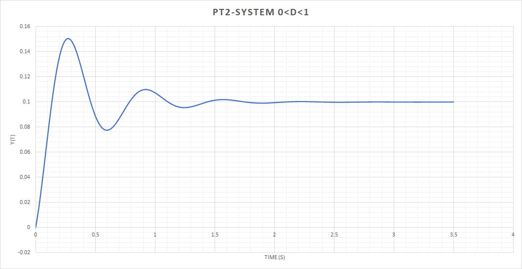
Because 0 < D < 1 the system oscillates which can be seen in Figure 5. The Figure shows the System’s answer to a step input with 300 N. The stationary output of the system can be calculated by setting all derivatives to 0 and solve for x (just 0.001*300 in this case). The analytical solution of the ODE necessary to plot Figure 5 is not covered in this story.

Summary

Modeling technical systems is an important skill for engineers that is used in many different fields of application e.g. in FEA or Multibody Dynamics. Modeling a system consists basically of two aspects, the mathematical description of the system and the estimation of the degree of detail necessary to approximate the system properly. The mathematical aspect can be done in two different ways:

1. Setting up a block diagram
2. Setting up an ODE

Both methods lead to the same solution. The first method is commonly used to simulate dynamic systems with software like MATLAB/Simulink.

Author’s Notes

Thank you for reading this far! If you have any thoughts, annotations, or ideas about this story feel free to leave a comment.

References

1. Nollau, R. (2009). Modellierung und Simulation technischer Systeme: Eine praxisnahe Einführung. Heidelberg: Springer-Verlag Berlin Heidelberg. Retrieved on 17th of January from DOI 10.1007/978–3–540–89121–5